UDC 621.372, 532.59
INVESTIGATION OF MODERN NUMERICAL ANALYSIS METHODS OF SELF-OSCILLATORY CIRCUITS EFFICIENCY
A. M. Pilipenko, V. N. Biryukov
Southern Federal University
The paper is received on July 27, 2013
Abstract― In the paper the testing of numerical methods for analysis of oscillating systems in the time domain is performed. An oscillator’ differential equation with arbitrary polygonal nonlinearity was selected as a test problem. The high efficiency of trapezoidal method for analysis of self-oscillating circuits is shown.
Keywords: oscillating circuits, nonlinear differential equations, error analysis.
1. Introduction
Currently, there are many numerical methods for solving of ordinary differential equations (ODE) modeling the radio-frequency circuits in the time domain. The SPICE-like simulators and systems for engineering calculations Mathcad, Matlab used Gear method, based on the multistage backward differentiation formulas, one-step explicit and implicit multistage Runge-Kutta methods, and a number of other methods [1-3]. The choice of a numerical method is provided to the user. In turn, the methods have different accuracy, stability, complexity, so the wrong choice of method for solving ODE may lead to a sharp increase of the analysis time or even result in the failure of the program. These problems are most typical for the numerical analysis of the self-oscillating circuits in the time domain, since the ODE system describing such circuits is often oscillating and stiff simultaneously [3]. In the latter case, the efficiency of a method of numerical solution of ODE requires additional investigation.
The objective of this paper is a comparative analysis and evaluation of the effectiveness of modern methods for the numerical solution of ODEs of quite important class of circuits generating electrical signals close in shape to the harmonic.
The main model for the analysis of periodic oscillations in radio electronics is the Van der Pol equation obtained from the differential equation of RLC-circuit if the I-V characteristic of the nonlinear resistive element is approximated by the cubic polynomial [4, 5]. Unfortunately, getting an exact solution of the van der Pol is a laborious task [6].
If the current-voltage characteristic of the nonlinear element is approximated by a piecewise linear function, the exact solution can be obtained quite simple. Oscillator based on a polygonal nonlinearity is used below as test problem [7].
2. The oscillator's equation
Fig. 1 shows a circuit of the parallel-connected linear inductance, linear capacitance, and nonlinear resistive element with the current-voltage characteristic iG = f(v).
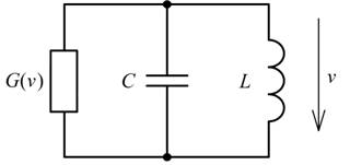
Fig. 1. The equivalent circuit of an electronic oscillator.
The system of differential equations for voltage and inductor current takes the form

The differential equation for the voltage takes the form

The circuit generates oscillations if differential
conductance ![]() is positive except for small v.
When approximating the current-voltage
characteristics of the nonlinear element
iG = f (v) by cubic polynomial equation
(2) gives rise to the Van der Pol.
The solution of this equation for the steady state is known [6].
Unfortunately, the explicit solution cannot be obtained, and there is benchmark
numerical solutions only specifically calculated with high accuracy for certain
parameters of the equation.
is positive except for small v.
When approximating the current-voltage
characteristics of the nonlinear element
iG = f (v) by cubic polynomial equation
(2) gives rise to the Van der Pol.
The solution of this equation for the steady state is known [6].
Unfortunately, the explicit solution cannot be obtained, and there is benchmark
numerical solutions only specifically calculated with high accuracy for certain
parameters of the equation.
3. The analytical solution of the oscillator
The analytical solution of the oscillator's equation for the stationary regime exists for piecewise linear approximation of the nonlinear conduction's I-V curve. One variety of such approximation is shown in Fig. 2. At each portion of the function variation v(t), which corresponds to a linear section of the I-V curve, the solution can be written as
Here ![]() ,
, ![]() at
at
![]() and
and
![]() otherwise.
For a periodic solution reference point can be chosen arbitrarily. We assume
that in the first time region
otherwise.
For a periodic solution reference point can be chosen arbitrarily. We assume
that in the first time region ![]() solution
v1(t) changes from –V0 to V0
and at the edges of interval
solution
v1(t) changes from –V0 to V0
and at the edges of interval ![]() the second portion v2(t) is equal to V0. The function v(t)
over the second half of the period T repeats the solution v(t)
at the first half of the period with the opposite sign and T/2 time delay.
the second portion v2(t) is equal to V0. The function v(t)
over the second half of the period T repeats the solution v(t)
at the first half of the period with the opposite sign and T/2 time delay.
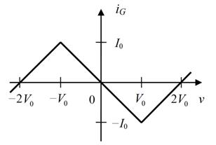
Fig. 2. V-A curve of the nonlinear resistive element.
The solution of Eq. (2) contains six unknowns, since in addition to the integration constants A1,1, A1,2, A2,1, A2,2 the period T and the boundary T0 between v1(t) and v2(t) needs to be found. To determine the unknown boundaries T0 and T we use continuity of inductance current, voltage of capacitance and function f (v) resulting derivative of the solution dv(t)/dt is also continuous. Stationary solution of Eq. (2) thus can be obtained by the system of algebraic equations as

Expression (3) can be used for real and complex values of sk. In the latter case, to simplify the solution of the system (4) it is expedient to define only the first complex integration constant, apart from a second one to be complex conjugate of the first constant.
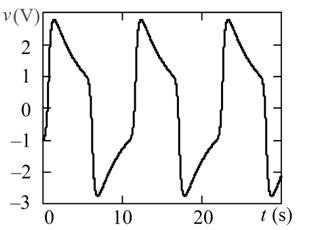
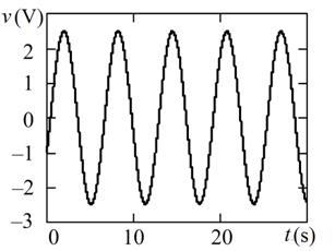
The stationary solutions of (2) obtained by the equations (3) and (4) are shown in Fig. 3. The solution in Fig. 3a is obtained for L = 1 H, C = 1 F, V0 = 1 V, I0 = 4 A. The solution in Fig. 3b is obtained for L = 1 H, C = 1 F, V0 = 1 V, I0 = 0.05 A. The shape of received oscillations is determined by the LC-tank factor Q = σ/G, where σ = (C/L)1/2 and G = I0 /V0. In the case shown in Fig. 3a Q = 0.25 < 1/2 and there are relaxation oscillations. Fig. 3b corresponds to the value of Q = 20 >>1/2, when the solution of equation (2) is close to sinusoidal oscillation.
|
|
|
a) b)
Fig. 3.The overdamped (a) and underdamped (b) oscillations.
4. Testing of numerical methods for solving ODE
This paper presents the results of a comparative analysis of the three methods - trapezoids, Gere and RADAU5. As a test task, the system (1) was used where f(v) is represented as a symmetrical piecewise linear function shown in Fig. 2.
Trapezoidal method is one of the simplest implicit methods for the numerical solution of ODE used in all electronic simulators. The stability region of trapezoidal method coincides with the left complex half-plane, and the global error of the method decreases with the square of the time step. Trapezoidal method for ODE system dx/dt = f (x, t), x(0) = x0 is described by the following difference scheme
where h is the time step, xn and xn + 1 - values of the solution of ODE in moments of time tn and tn + 1 = tn + h respectively. Trapezoidal method is an implicit Runge-Kutta method having a number of stages s = 1, and the order of accuracy p = 2.
Gear's method is the primary method of analysis of transients in electronic simulators. Gear's method is implemented using an algorithm that provides automatic selection of the time steps and order of method, depending on the specified error. Difference scheme of the Gear method is implicit multistep formula, known as backward differentiation formula [1]. BDF-formulae are used in practice of the order accuracy of the first to sixth.
RADAU5 is one of the most perspective Runge-Kutta methods [2]. The RADAU5 method is based on a three-stage fully implicit Runge-Kutta method of the fifth order of accuracy. RADAU5 method requires solving a system of algebraic equations with the dimension of three times higher than dimension of ODE of specified circuit.
To assess the effectiveness of the above-described numerical methods we use here the methodology proposed in [9]. As a criterion for the efficiency of the method we will use the accuracy of the basic parameters estimation of generated oscillations – the frequency and amplitude. The current relative estimation errors of frequency and amplitude are determined using the following relations respectively
 ,
,  .
.
Here ω(t) and Am(t) are assessments of the frequency and amplitude of the oscillations derived from the solution of (1) by numerical methods; ω0 and Am0 are the exact values of the same parameters obtained on the basis of (3) and (4).
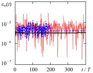
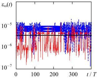
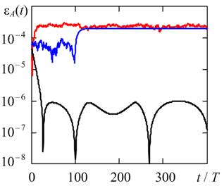
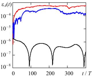
Fig. 4 and Fig. 5 show the relative estimation errors of frequency and amplitude of stationary oscillations at two oscillating system quality factor Q = 20 and Q = 100. The system of equations (1) was carried out numerically at a predetermined maximum time step hmax = T/1000, where T = 2π/ω0 - oscillation period.
The calculated values of frequency and amplitude of the oscillations:
a) Q = 20 (L = 1 H, С = 1 F, V0 = 1 V, I0 = 0.05 А):
ω0 = 0.99989149411682 rad/s, Am0 = 2.475477417618089 V;
b) Q = 100 (L = 1 H, С = 1 F, V0 = 1 V, I0 = 0.01 А):
ω0 = 0.99999565970188 rad/s, Am0 = 2.475416990116814 V.
|
|
|
a) b)
Fig. 4. The time variation of the relative error of frequency in the solution (1) by methods of trapezoids, BDF, and RADAU5. a) Q = 20, b) Q = 100.
|
|
|
a) b)
Fig. 5. Time variation of the relative error of the amplitude in the solution (1) by methods of trapezoids, BDF, and RADAU5. a) Q = 20, b) Q = 100.
To assess the period of oscillation the linear interpolation of numerical solution at the points of v(t) changes sign was used. To estimate the amplitude the quadratic interpolation is of v(t) was used at the points of local extremes. The initial conditions were v(0) = Am0 , i(0) = 0. A monitoring interval is selected so as to show the onset of steady state.
Fig. 4 shows for all the considered numerical methods the estimating of the frequency error has the same order of magnitude. In turn, as shown in Fig. 5, the estimating of the amplitude error for the method of the trapezoids is about two orders of magnitude less than similar error of Gear and RADAU5 due to the P-stability of trapezoids [10].
5. Conclusions
Results of the numerical analysis methods testing for self-oscillating circuit in the time domain were obtained to compare the accuracy of analysis results by various methods. The oscillator with a nonlinear element having a piecewise linear current-voltage characteristics was considered as a test the problem. This task is important for practice, because the discontinuity of derivatives of the solution in oscillatory systems is possible not only by reason of the method of approximation of V-A curve but also occurs in the analysis of high-Q circuits working in current mode of the cut-off [11].
APPENDIX
Half-period’s numerical solution

a) Q = 20:
T0 = 0.8317421985141854; T = 6.283867143733802;
A1 = –
0.5 – j∙1.11864478698996; A3 = –
0.54009929904588 – j∙1.18335071450520; A2 = ![]() ; A4 =
; A4 = ![]() ; s1 =
0.025 +
; s1 =
0.025 + ![]() ;
; ![]() ;
s3 = – s2;
;
s3 = – s2; ![]() .
.
b) Q = 100:
T0 = 0.831712434098467; T = 6.2832125781953;
A1 = – 0.5 – j∙1.1294252349926; A3 = – 0.50788674459494 – j∙1.14224014922639;
A2 = ![]() ; A4 =
; A4 = ![]() ; s1 =
0.005 +
; s1 =
0.005 + ![]() ;
; ![]() ;
s3 = – s2;
;
s3 = – s2; ![]() .
.
References
1. Hairer E., Nørsett S. P., Wanner G. Solving Ordinary Differential Equations I. Nonstiff Problems, Springer, 1993.
2. Hairer E., Wanner G. Solving Ordinary Differential Equations II. Stiff and Differential-Algebraic Problems, Springer, 1996, Springer, 1993.
3. Pilipenko A. M., Biryukov V. N. Hybrid Methods for Solution of Ordinary Differential Equations of Stiff and/or Oscillating Circuits. Radio Engineering, No 1, 2011, pp. 11-15 (in Russian)
4. Kuznetsov A.P., Kuznetsov S. P., Ryskin N. M. Nonlinear vibrations. Textbook for high schools. Moscow, Publishing house of physical and mathematical literature, 2002 (in Russian).
5. Guzhev D. S., Kalitkin N. N. Burgers equation - a test for numerical methods. Mathematical modeling, 1995, Vol. 7, No 4, pp. 99 – 127 (in Russian).
6. Abd El-Halim Ebaid. Approximate periodic solutions for the non-linear relativistic harmonic oscillator via differential transformation method. Communications in Nonlinear Science and Numerical Simulation, 2010, v. 15, No. 7, pp. 1921-1927.
7. Biryukov V. N., Gatko L. E. Exact stationary solution of the oscillator nonlinear differential equation. Nonlinear World, Vol. 10, No. 9, 2012, pp. 613-616 (in Russian)
8. Andronov A. A., Vitt A. A., Chaikin S. E. Theory of oscillations. Moscow. State Publishing House of Physical and Mathematical Literature, 1959 (in Russian).
9. Biryukov V. N., Pilipenko A. M, Kovtun D. G. Estimation of the Numerical Methods’ Accuracy of Oscillating Differential Equations Analysis in Time-Domain. Radio Engineering, No 9, 2011, pp. 104-107 (in Russian)
10. Petzold L. R., Jay L. O., Yen J. Numerical solution of highly oscillatory ordinary differential equations. Acta Numerica, 1997, pp. 437 – 483.
11. Pietrenko W., Janke W., Kazimierczuk A. K. Large-signal time-domain simulation of class E amplifier. IEEE International Symposium in Circuits and Systems, ISCAS 2002, v.5, p. 21 – 24.