NEAR – FIELD COHERENT EFFECTS AT THERMAL MICROWAVE RADIATION RECEIVING ON COUPLED LINEAR WIRE ANTENNAS
Y. N.
Barabanenkov1, M. Yu. Barabanenkov2, V. A. Cherepenin1
1 V.A. Kotelnikov Institute of Radioengineering and Electronics of RAS, Moscow
2 Institute of Microelectronics Technology of RAS, Chernogolovka
Received December 4, 2011
Ближнеполевые когерентные эффекты при приеме теплового микроволнового излучения взаимодействующими линейными проволочными антеннами
Ю. Н. Барабаненков1, М. Ю. Барабаненков2, В.
А. Черепенин1
1 Институт радиотехники и электроники им. В.А. Котельникова РАН, Москва
2 Институт проблем технологии микроэлектроники и особочистых материалов РАН, Черноголовка
Abstract. We apply to study coupled receiving antennas a theory of electromagnetic wave multiple scattering by ensemble of dielectric and conductive bodies, with describing the excited currents inside bodies in terms of electric field tensor T-scattering operator. A system of equations for currents on surfaces of coupled perfectly conductive receiving antennas is written with the aid of a single antenna surface T-scattering operator. This system is resolved for the case of coupled linear wire receiving antennas in the form of thin vibrator-dipoles when asymptotic method of “big logarithm“ leads to separable wire T-scattering operator of single tuned vibrator-dipole. The separability simplifies analytic evaluating the local total currents on two (and more) coupled receiving antennas and get a dimensionless coupling factor. Our final aim consists in using the obtained analytic solution to study near field coherent effects caused by thermal microwave radiation incident electric field distribution along single or two coupled receiving vibrator-dipole antennas placed at a heated biological object boundary surface and tuned to half wavelength in the object. In the case of equilibrium thermal radiation we meet a generalized Nyquist formula for currents’ fluctuations excited on coupled receiving vibrator-dipole antennas, with accounting the auto-correlation and cross-correlation functions of random electric field inside each antenna and on both antennas, respectively. In the case of local volume change of the biological object temperature distribution we reveal in the model framework of random electric dipole source inside object absorption skin slab area the interference-extreme properties for fluctuations of currents excited along antennas depending on relative positions of antennas and random electric dipole source. The reveled extreme properties are used as base to reconstruct the random electric dipole position via scanning the single antenna or two coupled ones along biological object boundary surface.
Key words: receiving coupled antennas, excited currents, T- scattering operator, thin vibrator antennas, biological object, temperature local variation, thermal radiation, interference receiving fields, scanning local random source.
Аннотация. Мы применяем теорию многократного рассеяния электромагнитных волн на ансамбле диэлектрических и проводящих тел для изучения взаимодействующих принимающих антенн, описывая возбужденные внутри антенн токи с помощью тензорного T –оператора рассеяния электрического поля. Система уравнений для токов на поверхностях взаимодействующих металлических принимающих антенн записывается с помощью поверхностного T- оператора рассеяния изолированной антенны. Записанная система решается для случая взаимодействующих линейных проволочных принимающих антенн в форме тонких вибраторов – диполей асимптотическим методом “ большого логарифма “, приводящим к сепарабельному линейному T- оператору рассеяния изолированного настроенного вибратора-диполя. Сепарабельность упрощает аналитическое вычисление локальных токов на двух ( и более) взаимодействующих антеннах и безразмерного параметра взаимодействия антенн. Наша окончательна цель состоит в использовании полученного аналитического решения к изучению ближнеполевых когерентных эффектов, обусловленных распределением падающего электрического поля теплового микроволнового излучения вдоль изолированного или двух взаимодействующих принимающих вибраторов-диполей, расположенных около граничной поверхности нагретого биологического объекта и настроенных на половину длины волны в объекте. При равновесном тепловом излучении мы приходим к обобщенной формуле Найквиста для флуктуаций токов, наведенных на взаимодействующих принимающих вибраторах-диполях, с учетом авто-корреляционной и кросс-корреляционной функций случайного электрического поля на каждом или обоих вибраторах-диполях, соответственно. Рассматривая локальное объемное изменение распределения температуры биологического объекта, мы обнаруживаем в рамках модели случайного электрического дипольного источника внутри поглощающего скин-слоя объекта интерференционно-экстремальные свойства возбуждаемых вдоль принимающих вибраторов – диполей флуктуационных токов в зависимости от относительного расположения вибраторов-диполей и случайного электрического дипольного источника теплового излучения. Обнаруженные экстремальные свойства используются как основа для восстановления расположения случайного электрического дипольного источника путем сканирования изолированным или двумя взаимодействующими принимающими вибраторами-диполями вдоль граничной поверхности биологического объекта.
Ключевые слова: принимающие взаимодействующие антенны, возбужденные токи, T- оператор рассеяния, тонкая вибраторная антенна, биологический объект, локальная вариация температуры, тепловое излучение, интерференция принимаемых полей, сканирование локального случайного источника.
Introduction
Measuring method of the temperature spatial distribution inside of a biological tissue object by recording its own thermal radiation in the microwave range is well known at the present time [1]. During the last twenty years, there has been realized that a contact antenna [2-4] or system of contact antennas [5] are situated in the area of a heated object thermal near fields, which have basically the form of evanescent electromagnetic waves exponentially decaying in perpendicular to the object boundary surface direction accordingly with Rytov’s prediction [6].
Note, mean size ![]() of a contact antenna aperture is rationally
to be chosen in accordance with [2-5] as being much smaller than radiation
wavelength
of a contact antenna aperture is rationally
to be chosen in accordance with [2-5] as being much smaller than radiation
wavelength ![]() in free space and of the order of the radiation
wavelength
in free space and of the order of the radiation
wavelength ![]() inside a biological object, i.e.,
inside a biological object, i.e., ![]() . Such inequalities suppose the real part
. Such inequalities suppose the real part ![]() of biological tissue complex dielectric permittivity
of biological tissue complex dielectric permittivity
![]() in microwave range to be substantially
greater the dielectric permittivity
in microwave range to be substantially
greater the dielectric permittivity ![]() of free space that is
really the case for some tissues. For example, the dielectric permittivity of
human head brain may be taken at frequency
of free space that is
really the case for some tissues. For example, the dielectric permittivity of
human head brain may be taken at frequency ![]() = 780 MHz
to be
= 780 MHz
to be ![]() [5] that gives
[5] that gives ![]() =
39 cm,
=
39 cm, ![]() =
7 cm and absorption skin depth
=
7 cm and absorption skin depth ![]() =
= ![]() = 4 cm where
= 4 cm where ![]() =
= ![]() =
= ![]() is the
complex wave number inside brain medium, with
is the
complex wave number inside brain medium, with ![]() =
= ![]() and
and ![]() =
= ![]() . Under above inequalities putting on mean
size aperture, the contact antenna receives strong decaying evanescent waves of
thermal radiation in free space, which correspond to weak decaying evanescent
waves inside biological object.
. Under above inequalities putting on mean
size aperture, the contact antenna receives strong decaying evanescent waves of
thermal radiation in free space, which correspond to weak decaying evanescent
waves inside biological object.
The wave theory [6,7,8] of an absorbing body thermal electromagnetic radiation having been published , Levin and Rytov [9] and Rytov et al [10] have considered some problems on current excitation in metallic antennas by thermal radiation fields, including the case of thin metallic antennas (linear wire antennas). To considered problems are related: (i) antenna excitation in equilibrium thermal radiation field; (ii) current excitation in antenna by thermal radiation of distant bodies; (iii) current excitation in coupled antennas, with phenomenological accounting of coupling effect by antenna mutual impedance.
The aim of our presented work is to consider the current excitation in coupled receiving antennas by incident electromagnetic field, with evaluating the coupling effect via analytic solution to system of equations for currents’ distribution on coupled linear wire tuned antennas. Especially we intend to study the current excitation in such antennas by thermal radiation of small body placed in near field zone of antennas, as well as by equilibrium thermal radiation. Actually our work consists in the following.
Because electromagnetic mutual interaction
(coupling) the antennas is included in theory of wave multiple scattering by
ensemble of bodies [11], we write the volume current density inside a body in
terms of the body electric field tensor T-scattering operator [12-17] and then
derive the general system of equations for volume current densities inside all
bodies of ensemble ones with the aid of Watson composition rule [12,
15] for
scattering operators. A specific property of the derived system of equations
for currents’ densities inside bodies consists in that the system is written in
terms of single body T-scattering operator. In particular case of antennas
placed at a heated biological object boundary surface the derived general system
of equations for volume currents’ densities inside antennas takes into account
also the coupling effects between antennas and object boundary surface
(inhomogeneous object) that we do neglect in our concrete calculations. What
is more, bearing in mind that mean size ![]() of
contact antennas conforms to wavelength
of
contact antennas conforms to wavelength ![]() inside
a biological object, we think them as were placed in the object boundary subsurface,
with thickness being not more or order the absorption skin depth
inside
a biological object, we think them as were placed in the object boundary subsurface,
with thickness being not more or order the absorption skin depth ![]() . On the way of such simplifications the
mentioned general system of equations is transformed to a reduced system of
equations for surface currents’ densities on surfaces of coupled perfectly
conducting receiving antennas written with the aid of a single antenna surface T-scattering
operator. The reduced system supposes all coupled antennas to be placed in an effective
unbounded medium, with wave number being equal to wave number
. On the way of such simplifications the
mentioned general system of equations is transformed to a reduced system of
equations for surface currents’ densities on surfaces of coupled perfectly
conducting receiving antennas written with the aid of a single antenna surface T-scattering
operator. The reduced system supposes all coupled antennas to be placed in an effective
unbounded medium, with wave number being equal to wave number ![]() inside the biological object under study.
The next our step consists in passing to linear wire antennas, with mean
diametrical size
inside the biological object under study.
The next our step consists in passing to linear wire antennas, with mean
diametrical size ![]() of each wire being very small
compared to wire length
of each wire being very small
compared to wire length ![]() and wavelength
and wavelength ![]() ,
, ![]() ;
; ![]() . Passing to linear wire replaces the
above single antenna surface T-scattering operator to single wire T-scattering
operator that is one-dimensional kernel, which expresses the total current in a
cross section of the wire through excited electric field component along wire. According
to Levin and Rytov [9], the single wire T-scattering operator of tuned linear
wire antenna,
. Passing to linear wire replaces the
above single antenna surface T-scattering operator to single wire T-scattering
operator that is one-dimensional kernel, which expresses the total current in a
cross section of the wire through excited electric field component along wire. According
to Levin and Rytov [9], the single wire T-scattering operator of tuned linear
wire antenna, ![]() (
(![]() is
integer number), takes a simple separable form in asymptotic limit of “big
logarithm” when parameter
is
integer number), takes a simple separable form in asymptotic limit of “big
logarithm” when parameter ![]() has a small value.
Theory of this asymptotic limit was elaborated by Leontovich and Levin [18]
after Hallen paper [19] for analytic solution to Pocklington integral equation
[20] that describes the current distribution along linear wire antenna
depending on excited electric field component along the wire. We use the separable
form of the single wire scattering operator to resolve the system of equations
for currents’ distributions along two coupled tuned linear wire antennas in
terms of excited electric field components along both wires and their coupling
factor, which is defined as ratio of antenna mutual impedance to self-impedance
of a single antenna and evaluated directly. The mutual impedance of two wire
antennas was studied earlier [21, 22] for transmitting antennas with the aid of
more complicated method; convenient formulas for mutual impedance of antennas
placed on big distant between them are considered in paper [23]. The obtained currents’
distributions along coupled tuned linear wire antennas are applied to the case when
exciting electric field is caused by thermal radiation of a biological object,
with temperature being equal to sum of homogeneous component
has a small value.
Theory of this asymptotic limit was elaborated by Leontovich and Levin [18]
after Hallen paper [19] for analytic solution to Pocklington integral equation
[20] that describes the current distribution along linear wire antenna
depending on excited electric field component along the wire. We use the separable
form of the single wire scattering operator to resolve the system of equations
for currents’ distributions along two coupled tuned linear wire antennas in
terms of excited electric field components along both wires and their coupling
factor, which is defined as ratio of antenna mutual impedance to self-impedance
of a single antenna and evaluated directly. The mutual impedance of two wire
antennas was studied earlier [21, 22] for transmitting antennas with the aid of
more complicated method; convenient formulas for mutual impedance of antennas
placed on big distant between them are considered in paper [23]. The obtained currents’
distributions along coupled tuned linear wire antennas are applied to the case when
exciting electric field is caused by thermal radiation of a biological object,
with temperature being equal to sum of homogeneous component ![]() and temperature local volume spatial
variation
and temperature local volume spatial
variation![]() . The homogeneous component of the object
temperature
. The homogeneous component of the object
temperature ![]() creates an equilibrium thermal radiation
that is characterized by standard form [10] of electric field spatial correlation
function as electric field tensor Green function imaginary part, with a scalar
factor being in front of it. A local volume variation of the object temperature
creates an equilibrium thermal radiation
that is characterized by standard form [10] of electric field spatial correlation
function as electric field tensor Green function imaginary part, with a scalar
factor being in front of it. A local volume variation of the object temperature
![]() gives rise to the thermal radiation from
corresponding local random electric current density variation
gives rise to the thermal radiation from
corresponding local random electric current density variation ![]() (dipole) delta-correlated with respect to
spatial position and polarization (orientation). Such electric current
(dipole) delta-correlated with respect to
spatial position and polarization (orientation). Such electric current ![]() can be thought as sum of three mutually
perpendicular and statistically independent random currents (dipoles). On this
way we come to a model of random electric dipole source inside a biological
object oriented parallel to coupled tuned linear wire antennas. We suppose the
random dipole to be placed in near wave zone of both antennas and evaluate the antennas’
excitation via this dipole with the aid of method elaborated by Brilliouin [24],
Pistolkors [25], and Bechmann [26] to study electromagnetic field in near zone
of linear wire antenna (see also [27]). This model of random electric dipole source
reveals the interference – extreme properties for fluctuations of excited in
antennas currents depending on relative positions of antennas and the random
dipole source. The revealed interference – extreme properties are analyzed from
viewpoint to reconstruct the random dipole source position via special
arrangement of two antennas on biological object boundary surface or via
special scanning the single antenna along this boundary surface.
can be thought as sum of three mutually
perpendicular and statistically independent random currents (dipoles). On this
way we come to a model of random electric dipole source inside a biological
object oriented parallel to coupled tuned linear wire antennas. We suppose the
random dipole to be placed in near wave zone of both antennas and evaluate the antennas’
excitation via this dipole with the aid of method elaborated by Brilliouin [24],
Pistolkors [25], and Bechmann [26] to study electromagnetic field in near zone
of linear wire antenna (see also [27]). This model of random electric dipole source
reveals the interference – extreme properties for fluctuations of excited in
antennas currents depending on relative positions of antennas and the random
dipole source. The revealed interference – extreme properties are analyzed from
viewpoint to reconstruct the random dipole source position via special
arrangement of two antennas on biological object boundary surface or via
special scanning the single antenna along this boundary surface.
The organization of the paper is as follows. In Sec.2 the general equations’ system for volume currents’ densities inside coupled receiving antennas near biological object boundary surface is written in terms of a single antenna electric field tensor T –scattering operator. In Sec.3 the derived general system is transformed to reduced system of equations for surface currents on perfectly conducting antenna’s surfaces written in terms of a single antenna surface T- scattering operator. In Sec. 4 a passing to system equations for currents along coupled linear wire antennas is described and these equations’ system is written in terms of a single wire T-scattering operator. In Sec. 5 the equations’ system for currents along two coupled turned linear wire antennas is resolved in asymptotic limit of the so-called “big logarithm”. In Sec. 6 the obtained currents’ distributions along coupled tuned linear wire antennas is applied to the problem of antennas’ exciting by a biological object thermal radiation via the object temperature homogeneous component. In Sec. 7 a local volume variation of the object temperature is modeled by corresponding random electric dipole source and the interference- extreme properties for fluctuations of excited in antennas’ currents depending of relative positions of antennas and the random dipole source are considered. Conclusions are made in Sec. 8.
Coupled receiving antennas at biological object boundary
We start with the Helmholtz
vector wave equation for electric field ![]() of a
monochromatic electromagnetic wave of frequency
of a
monochromatic electromagnetic wave of frequency ![]() in a three
-dimensional (
in a three
-dimensional (![]() ) inhomogeneous isotropic
dielectric and conducting structure writing the equation as
) inhomogeneous isotropic
dielectric and conducting structure writing the equation as

|
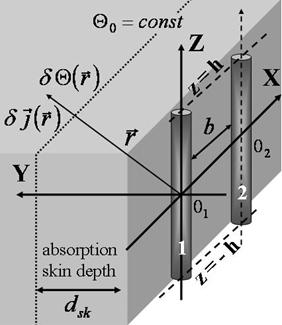
Figure
1. Schematic showing of biological object (grey area; dotted line
symbolically visualizes an absorption skin depth |
Our
structure consists of homogeneous biological object occupying (Fig. 1) the left
half space ![]() > 0 of the Cartesian coordinate system
> 0 of the Cartesian coordinate system
![]() and receiving antennas placed at the
object boundary surface
and receiving antennas placed at the
object boundary surface ![]() = 0. Symbol
= 0. Symbol ![]() denotes the complex dielectric
permittivity of the structure without antennas (bounded biological object)
equal to dielectric permittivity
denotes the complex dielectric
permittivity of the structure without antennas (bounded biological object)
equal to dielectric permittivity ![]() = 1 in free space
= 1 in free space ![]() < 0
and
< 0
and ![]() inside biological object
inside biological object ![]() > 0, with
> 0, with ![]() and
and ![]() being real part of the complex dielectric
permittivity and specific conductivity of the object, respectively. An
effective “scattering potential”
being real part of the complex dielectric
permittivity and specific conductivity of the object, respectively. An
effective “scattering potential” ![]() of antennas is defined
by
of antennas is defined
by

where ![]() is the complex dielectric permittivity of
antenna, with
is the complex dielectric permittivity of
antenna, with ![]() and
and ![]() being
its real dielectric permittivity and specific conductivity, respectively. The
function
being
its real dielectric permittivity and specific conductivity, respectively. The
function ![]() is the characteristic function of the
is the characteristic function of the ![]() -th antenna, equal to unity if point
-th antenna, equal to unity if point
![]() belongs to the region occupied by the
belongs to the region occupied by the ![]() -th antenna and equal to zero otherwise.
The antennas are assumed to be identical and centered at positions
-th antenna and equal to zero otherwise.
The antennas are assumed to be identical and centered at positions ![]() ,
, ![]() . Each antenna
is characterized by a single scattering potential
. Each antenna
is characterized by a single scattering potential ![]() ,
defined via Eq.(2). The magnetic permittivity is supposed to be
,
defined via Eq.(2). The magnetic permittivity is supposed to be ![]() everywhere. The vector
everywhere. The vector ![]() denotes the electromagnetic field source
volume current density, which can be random as in the case of biological object
thermal radiation. The summation over repeated Greek subscripts is implied in
the limits from 1 to 3, with 1, 2, 3 corresponding to the
denotes the electromagnetic field source
volume current density, which can be random as in the case of biological object
thermal radiation. The summation over repeated Greek subscripts is implied in
the limits from 1 to 3, with 1, 2, 3 corresponding to the ![]() axes. The Gaussian system of units is
used and
axes. The Gaussian system of units is
used and ![]() denotes the light speed in the free space.
denotes the light speed in the free space.
We are interested in the electric currents excited inside antennas. Let us introduce a vector

that presents
accurate with the factor ![]() a sum
a sum ![]() of volume conducting and displacement
current densities inside the
of volume conducting and displacement
current densities inside the ![]() -th antenna. A complete
current density
-th antenna. A complete
current density ![]() excited in all antennas can be
evaluated, provided the electric field tensor
excited in all antennas can be
evaluated, provided the electric field tensor ![]() -scattering
operator
-scattering
operator ![]() [16,17] of antennas’ system is known . Really,
denote
[16,17] of antennas’ system is known . Really,
denote ![]() the electric field retarded Green tensor
function of the bounded biological object, which satisfies the Helmholtz Eq.(1)
without antenna scattering potential in the left-hand side (LHS) and with the
delta-source term
the electric field retarded Green tensor
function of the bounded biological object, which satisfies the Helmholtz Eq.(1)
without antenna scattering potential in the left-hand side (LHS) and with the
delta-source term ![]() in the right-hand side (RHS) of
the equation and the radiation conditions in the infinity. The electric field
Green tensor function
in the right-hand side (RHS) of
the equation and the radiation conditions in the infinity. The electric field
Green tensor function ![]() enables one to bring [15-17] a
solution problem for the Helmholtz Eq.(1) to wave integral equation
enables one to bring [15-17] a
solution problem for the Helmholtz Eq.(1) to wave integral equation
Here ![]() denotes the incident on antennas electric
field given by
denotes the incident on antennas electric
field given by

Solution
to the wave integral Eq.(4) is presented [15-17] in terms of the electric field
tensor ![]() -scattering operator of antennas’ system by
an equality that has a form
-scattering operator of antennas’ system by
an equality that has a form
Comparison
of this equality with integral Eq.(4) gives the Lippmann- Schwinger equation for
the electric field ![]() - scattering operator of antennas’
system
- scattering operator of antennas’
system
![]() (7)
(7)
and a symbolic
operator relation ![]() , which in details is written as
, which in details is written as
The
obtained relation shows that one can indeed evaluate the complete current
density excited in all antennas, having known the electric field tensor ![]() - scattering operator of antennas’ system
and the incident on antennas electric field.
- scattering operator of antennas’ system
and the incident on antennas electric field.
The wave integral Eq. (4) can be derived with the aid of vector Green theorem and the boundary conditions on antennas surfaces and at infinity, with similar to [16] manipulating for the case of bodies’ system in free space.
Side by side with the electric
field ![]() -scattering operator of antenna’s system
it is convenient to consider also the electric field
-scattering operator of antenna’s system
it is convenient to consider also the electric field ![]() -scattering
operator of a single
-scattering
operator of a single ![]() -th antenna
-th antenna ![]() , that satisfies the Lippmann-Schwinger
equation with the single scattering potential,
, that satisfies the Lippmann-Schwinger
equation with the single scattering potential, ![]()
![]() . According to Watson composition rule
[12,15] connection between
. According to Watson composition rule
[12,15] connection between ![]() - scattering operator
of antenna’s system and single scattering operators
- scattering operator
of antenna’s system and single scattering operators ![]() of
antennas is given by a system of operator equations
of
antennas is given by a system of operator equations
Here ![]() has sense of
has sense of ![]() -
scattering operator of
-
scattering operator of ![]() -th antenna coupled with
all other antennas. Convolving Eq.(9) with the incident electric field
-th antenna coupled with
all other antennas. Convolving Eq.(9) with the incident electric field ![]() gives for current densities
gives for current densities ![]() inside antennas (3) a basic system of
equations
inside antennas (3) a basic system of
equations
written
in terms of current densities inside of single antennas ![]() and
the single scattering operators
and
the single scattering operators ![]() of antennas.
of antennas.
The basis system of Eqs .(10) for currents’ densities inside antennas is too complicated, having accounting the coupling effect not only between antennas but also between antennas and bounded biological object. In the next section the system (10) is simplified via accounting the coupling effect between antennas only.
Coupled receiving perfectly conducting antennas inside the object boundary subsurface
Remind that in practice [2-5] the
mean size of contact antennas conforms to wavelength ![]() inside
a biological object. We use that conformity to avoid the problem of coupling
between antennas and biological object boundary, with replacing in all
equations of the preceding section the electric field Green tensor function
inside
a biological object. We use that conformity to avoid the problem of coupling
between antennas and biological object boundary, with replacing in all
equations of the preceding section the electric field Green tensor function ![]() of the bounded biological object to the
Green tensor function
of the bounded biological object to the
Green tensor function ![]() of unbounded biological object.
Simultaneously one needs replacing in Eqs. (2) and (3) the permittivity
of unbounded biological object.
Simultaneously one needs replacing in Eqs. (2) and (3) the permittivity ![]() to
to ![]() .
.
We consciously use such rather rough approach to focus our attention on coupling effects between antennas at receiving the biological thermal radiation.
The above electric field Green tensor function of unbounded biological object is given by

where ![]() denotes a scalar Green function. The
basic Eqs.(10) for currents densities
denotes a scalar Green function. The
basic Eqs.(10) for currents densities ![]() inside
two coupled antennas
inside
two coupled antennas ![]() takes a form
takes a form

and

where indices 1 and 2 are related to antennas 1 and 2 (Fig.1), respectively, and integrations are performed inside volumes of these antennas.
The next problem consists in
evaluating the single scattering operators ![]() and
and ![]() of antennas 1 and 2. Instead of direct solution
to the Lippmann- Schwinger equation for a single scattering operator mentioned
before a system of Eqs.(9), we remind an expression after Eqs.(10) for current
density inside a single scattering antenna in terms of its single scattering
operator and incident electric field, with rewriting the total electric field
(6) everywhere around and inside antenna as
of antennas 1 and 2. Instead of direct solution
to the Lippmann- Schwinger equation for a single scattering operator mentioned
before a system of Eqs.(9), we remind an expression after Eqs.(10) for current
density inside a single scattering antenna in terms of its single scattering
operator and incident electric field, with rewriting the total electric field
(6) everywhere around and inside antenna as
Resolving
this equation with respect to current density ![]() gives a
convenient tool to find the single scattering operator Green theorem of perfectly
conducting antenna. But previously to make so we need discussing some general
properties of Eq. (14) for a body with finite dielectric permittivity.
gives a
convenient tool to find the single scattering operator Green theorem of perfectly
conducting antenna. But previously to make so we need discussing some general
properties of Eq. (14) for a body with finite dielectric permittivity.
The integral Eq. (14) for
electric field![]() , with replacing
, with replacing ![]() to
to ![]() , is
known in wave multiple scattering theory for a long period of time and often
related to pioneering papers of Foldy [28] and Lax [29]. Nevertheless, an
opinion exists [30] that one needs verifying consistence the Eq. (14) with
boundary conditions on the body surface directly. In this connection we would
like to make the two following remarks.
, is
known in wave multiple scattering theory for a long period of time and often
related to pioneering papers of Foldy [28] and Lax [29]. Nevertheless, an
opinion exists [30] that one needs verifying consistence the Eq. (14) with
boundary conditions on the body surface directly. In this connection we would
like to make the two following remarks.
First, as was mentioned after Eq, (8), the Eq. (14) has been derived [16] with the aid of vector Green theorem and accounting the boundary conditions.
Second, Eq. (14) is a three-
dimensional singular integral equation and demands some accuracy at handling
with it. If point ![]() is placed inside the body one
has to take into account the strong singularity of the tensor Green function,
Eq. (11), at
is placed inside the body one
has to take into account the strong singularity of the tensor Green function,
Eq. (11), at ![]() , with decomposing [31-33] the one into a
delta Dirac function term
, with decomposing [31-33] the one into a
delta Dirac function term ![]() and principal part
and principal part ![]() where a constant tensor
where a constant tensor ![]() depends on the shape of the exclusion
domain chosen to define the principal part. If the exclusion domain is an infinitesimal
sphere the tensor
depends on the shape of the exclusion
domain chosen to define the principal part. If the exclusion domain is an infinitesimal
sphere the tensor ![]() Substituting the decomposed
tensor Green function into Eq. (14) gives after [32,34] an equation
Substituting the decomposed
tensor Green function into Eq. (14) gives after [32,34] an equation

where
integration in the RHS is performed over body volume, with excluding an
infinitesimally small spherical domain around point ![]() . A
local electric field
. A
local electric field ![]() and transformed scattering
potential
and transformed scattering
potential ![]() are defined by
are defined by
 (16)
(16)
The
strong singular term of the tensor Green function in Eq. (11) at ![]() and
and ![]() has a form
has a form
![]() and becomes of zero value by averaging over
unit vector
and becomes of zero value by averaging over
unit vector ![]() along vector
along vector ![]() directions.
Hence the integral in the sense of principal value in the RHS of Eq. (15) is
good defined one and can be expressed according to general theory of many
dimensional singular integrals [35] as sum of absolutely converged integrals.
However, Eq. (15) does not show directly its consistence with boundary
conditions. Therefore we transform this equation to a physically transparent
form usual for theory of electromagnetism [27].
directions.
Hence the integral in the sense of principal value in the RHS of Eq. (15) is
good defined one and can be expressed according to general theory of many
dimensional singular integrals [35] as sum of absolutely converged integrals.
However, Eq. (15) does not show directly its consistence with boundary
conditions. Therefore we transform this equation to a physically transparent
form usual for theory of electromagnetism [27].
Let us apply a lemma (see, e.g., [36], appendix 50) as the rule to bring out the second derivative outside the three dimensional singular integral
 (17)
(17)
where ![]() is some scalar test function. This lemma
enables one to transform Eq.(15) as follows
is some scalar test function. This lemma
enables one to transform Eq.(15) as follows
Here ![]() denotes the Hertz vector that is written
in terms of the body polarization vector
denotes the Hertz vector that is written
in terms of the body polarization vector ![]() as
as
 (19)
(19)
with
omitting the limit symbol at the RHS integral. The scalar electric potential ![]() is evaluated by applying the divergence
operator under integral sign in the RHS of Eq. (19). Then similar to the case
of dielectric polarization in electrostatics (see [27], paragraph 3.13) one can
introduce a volume density
is evaluated by applying the divergence
operator under integral sign in the RHS of Eq. (19). Then similar to the case
of dielectric polarization in electrostatics (see [27], paragraph 3.13) one can
introduce a volume density ![]() of body electric
polarization charge for point
of body electric
polarization charge for point ![]() inside the body and a
surface
inside the body and a
surface ![]() density one for point
density one for point ![]() on the body surface where
on the body surface where ![]() is the outward unit normal vector to the
surface. The surface charge is coursed by polarization vector discontinuity at
the body surface crossing and leads to discontinuity of the electric field (see
[27], paragraph 3.15) on the body surface according the equation
is the outward unit normal vector to the
surface. The surface charge is coursed by polarization vector discontinuity at
the body surface crossing and leads to discontinuity of the electric field (see
[27], paragraph 3.15) on the body surface according the equation
![]() (20)
(20)
where the
subscript plus and minus are related to regions out and inside the body at
surface point ![]() , respectively. Eq. (20) means
discontinuity the normal component of electric field at the body surface
crossing according to relation
, respectively. Eq. (20) means
discontinuity the normal component of electric field at the body surface
crossing according to relation ![]() as well as continuity
of electric field tangential component at the body surface crossing.
as well as continuity
of electric field tangential component at the body surface crossing.
Having verified the consistence
of Eq. (14) with the boundary conditions on the body surface, let us return to
system Eqs. (12) and (13) for currents’ densities inside two coupled antennas. In
the limit of a perfectly conducting antenna the current density inside its
volume becomes to be confined near the antenna surface ![]() .
Therefore we write, e.g.,
.
Therefore we write, e.g., ![]() where
where ![]() and
and ![]() are
elements of antenna volume and surface, respectively, as well as
are
elements of antenna volume and surface, respectively, as well as ![]() and
and ![]() are
antenna volume and surface current densities, respectively. We write similarly
a relation
are
antenna volume and surface current densities, respectively. We write similarly
a relation ![]() =
= ![]() defined
a surface
defined
a surface ![]() - scattering operator
- scattering operator ![]() . Substituting into Eqs. (12) and (13)
gives
. Substituting into Eqs. (12) and (13)
gives

and

Here the
indices 1 and 2 are related to antennas 1 and 2, respectively, but in deference
from Eqs.(12) and (13) the integrations are performed now along the surfaces of
antennas 1 and 2. Because the total electric field ![]() on
perfect conducting antenna’s surface is equal to zero the Eq.(18) takes a form
on
perfect conducting antenna’s surface is equal to zero the Eq.(18) takes a form
![]() (23)
(23)
if point ![]() is placed on the antenna 1 surface.
Resolving Eq.(23) with respect to the surface current density and bearing in
mind a relation
is placed on the antenna 1 surface.
Resolving Eq.(23) with respect to the surface current density and bearing in
mind a relation

one can
get the desired single surface ![]() - scattering operator
- scattering operator ![]() of antenna 1.
of antenna 1.
Coupled receiving linear wire antennas
Consider the case of linear wire
antennas in the form of thin vibrator- dipoles to be parallel to ![]() axis and occupying the regions
axis and occupying the regions ![]() as depicted in Fig.1. For a cylindrical vibrator
with diameter
as depicted in Fig.1. For a cylindrical vibrator
with diameter ![]() only tangential component
only tangential component ![]() of the surface current density
of the surface current density ![]() exists and one can introduce a total
current
exists and one can introduce a total
current ![]() in the cross-section
in the cross-section ![]() of the vibrator. Eq.(23) for the surface
current density of a single antenna is transformed in the case of linear wire
antenna under consideration to the Pocklington integral equation [20] (see also
[37])
of the vibrator. Eq.(23) for the surface
current density of a single antenna is transformed in the case of linear wire
antenna under consideration to the Pocklington integral equation [20] (see also
[37])
 (25)
(25)
with
vector potential ![]() -component
-component ![]() given by
given by
 (26)
(26)
Here ![]() as well as the observation
as well as the observation ![]() and source
and source ![]() points
are presented in cylindrical coordinates. The
points
are presented in cylindrical coordinates. The ![]() - component
of vector potential (26) is evaluated asymptotically for thin vibrator near
zone, where
- component
of vector potential (26) is evaluated asymptotically for thin vibrator near
zone, where ![]() and
and ![]() , as a
sum of logarithm’s and addition terms
, as a
sum of logarithm’s and addition terms
![]() (27)
(27)
with
addition term ![]() having a current functional
form
having a current functional
form
 (28)
(28)
Substituting
the vector potential ![]() - component asymptotics (27) into
Pocklington integral Eq.(25) leads to the Leontovich – Levin version [18] of Hallen integro-differential equation [19] (see also [37]) for current
distribution
- component asymptotics (27) into
Pocklington integral Eq.(25) leads to the Leontovich – Levin version [18] of Hallen integro-differential equation [19] (see also [37]) for current
distribution ![]() along single linear wire thin
vibrator-dipole receiving antenna
along single linear wire thin
vibrator-dipole receiving antenna

where current
functional ![]() is defined by
is defined by
 (30)
(30)
Remind
that ![]() is small parameter in asymptotic limit of
“big logarithm”.
is small parameter in asymptotic limit of
“big logarithm”.
Relation (24) between a single
antenna surface current density and antenna single surface ![]() - scattering operator takes in the limit
of linear wire thin vibrator –dipole antenna the form
- scattering operator takes in the limit
of linear wire thin vibrator –dipole antenna the form
 (31)
(31)
with a single
wire ![]() - scattering operator
- scattering operator ![]() defined by
defined by
 (32)
(32)
Similarly,
the system of Eqs. (21) and (22) for surface current densities of two coupled
antennas passes to equation system for current ![]() distributions
along two coupled linear wire antennas
distributions
along two coupled linear wire antennas ![]() = 1,2 written
in terms of single wire
= 1,2 written
in terms of single wire ![]() - scattering operators
- scattering operators ![]() as
as

and

Here ![]() where
where ![]() and
and ![]() is the distant between antennas (Fig. 1).
In the next section we present asymptotic solution to Leontovich – Levin-_Hallen
Eq.(29) and to equation system (33) and (34).
is the distant between antennas (Fig. 1).
In the next section we present asymptotic solution to Leontovich – Levin-_Hallen
Eq.(29) and to equation system (33) and (34).
Current distributions along two coupled tuned receiving linear wire antennas in the limit of “big logarithm”
Bearing in mind the small
parameter ![]() one can apply after [18] the perturbation
method of solution to Eq.(29) for current distribution
one can apply after [18] the perturbation
method of solution to Eq.(29) for current distribution ![]() along
single linear wire antenna in the form of expansion
along
single linear wire antenna in the form of expansion ![]() with
result of substitution
with
result of substitution
 (35)
(35)
 (36)
(36)
This system of equations should be resolved successively. We restrict ourselves by simple case of tuned vibrator-dipole.
The length ![]() of tuned vibrator – dipole is equal to
the whole multiple of half wavelength
of tuned vibrator – dipole is equal to
the whole multiple of half wavelength ![]() in the
biological object,
in the
biological object, ![]() or
or![]() , with
, with
![]() being integer. Eq.(35) for zero
approximation has a solution
being integer. Eq.(35) for zero
approximation has a solution![]() , where
, where ![]() is current amplitude and function
is current amplitude and function ![]() if
if ![]() is odd
and
is odd
and ![]() if
if ![]() is
even. Current amplitude
is
even. Current amplitude ![]() is defined by
orthogonality condition of zero approximation to RHS of Eq.(36) for the first
approximation that after some algebra gives
is defined by
orthogonality condition of zero approximation to RHS of Eq.(36) for the first
approximation that after some algebra gives
 (37)
(37)
The
quantity ![]() has sense of input impedance of single
vibrator – dipole feeding in the current maximum point, when
has sense of input impedance of single
vibrator – dipole feeding in the current maximum point, when ![]() and
and ![]() , and
it is evaluated via formula
, and
it is evaluated via formula

Here the
functions ![]() and
and ![]() are
defined by integrals
are
defined by integrals
 (39)
(39)
with ![]() being the integral sine [38] and regular
function
being the integral sine [38] and regular
function ![]() related to the integral cosine
related to the integral cosine ![]() and Euler constant
and Euler constant ![]() ≈ 0.5772 as
≈ 0.5772 as ![]() .
.
Substituting current distribution
![]() along turned single vibrator- dipole into
Eq.(31) gives for single wire
along turned single vibrator- dipole into
Eq.(31) gives for single wire ![]() - scattering operator
- scattering operator ![]() of such vibrator- dipole a separable
value defined by
of such vibrator- dipole a separable
value defined by
 (40)
(40)
The
separability property of single wire ![]() - scattering operator
makes the Eqs.(33) and (34) for current distributions along two coupled linear
wire antennas to be exactly resolved. One can write out result of this
resolution in a form similar to the case of a single linear wire antenna
putting
- scattering operator
makes the Eqs.(33) and (34) for current distributions along two coupled linear
wire antennas to be exactly resolved. One can write out result of this
resolution in a form similar to the case of a single linear wire antenna
putting ![]() where amplitudes
where amplitudes ![]() of
current distribution along two coupled linear wire antennas are given by
of
current distribution along two coupled linear wire antennas are given by

and

Here the
indices 1 and 2 are related to antennas 1 and 2, respectively, and integrations
are performed along these two antennas. A specific coupling factor ![]() where
where ![]() is
mutual impedance [37] of two vibrator - dipoles is defined by integral equality
is
mutual impedance [37] of two vibrator - dipoles is defined by integral equality
 (43)
(43)
Transforming double integral in this equality RHS by the method [25-26], with applying part by part integration, leads to a working formula for coupling factor evaluation
 (44)
(44)
where a
function ![]() is expressed in terms of integral cosine
and integral sine as
is expressed in terms of integral cosine
and integral sine as ![]() and parameters
and parameters ![]() and
and ![]() have a
form
have a
form
 (45)
(45)
|
Figure
2. Dependence of the real (solid line) and imaginary (dashed line) parts of
the specific coupling factor |
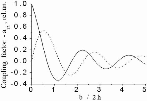
An useful
asymptotics for coupling factor ![]() at small distances
at small distances ![]() between antennas reads
between antennas reads

where input
impedance ![]() of single vibrator – dipole is defined by
Eq. (38). Fig.2 represents the real and imaginary parts of the coupling factor
of single vibrator – dipole is defined by
Eq. (38). Fig.2 represents the real and imaginary parts of the coupling factor ![]() versus the dimensionless distant
versus the dimensionless distant ![]() between two half wavelength
between two half wavelength ![]() vibrators.
vibrators.
In the next section we apply the presented currents’ distributions along single tuned vibrator- dipole as well as along two coupled tuned vibrator – dipoles to the problem of antennas’ exciting by a biological object thermal radiation via the object temperature homogeneous component.
Exciting single and coupled tuned receiving linear wire antennas by equilibrium thermal radiation
According to the general theory
[6] the electromagnetic thermal radiation of a heated absorbing body is created
by a random electric volume current density ![]() with
the spatial correlation function spectral density given by
with
the spatial correlation function spectral density given by

where ![]() denotes the body temperature multiplied
by the Boltzmann constant. In this section we are interesting in effects of
homogeneous component
denotes the body temperature multiplied
by the Boltzmann constant. In this section we are interesting in effects of
homogeneous component ![]() of the biological object
temperature. In this case one obtains from Eqs. (5), (11) and (47) the
following expression for the incident on antennas random electric field spatial
correlation function spectral density
of the biological object
temperature. In this case one obtains from Eqs. (5), (11) and (47) the
following expression for the incident on antennas random electric field spatial
correlation function spectral density

that is a standard form [10] of equilibrium thermal radiation electric field spatial correlation function spectral density.
Apply first the expression in Eq.
(48) to the case of a single tuned vibrator-dipole antenna exciting by a
biological object thermal radiation via object temperature homogeneous
component. Eq. (37) gives for the fluctuations’ spectral density ![]() of current distribution along receiving
antenna amplitude an equality
of current distribution along receiving
antenna amplitude an equality
 (49)
(49)
where one sees in the RHS integrand the auto- correlation function of random electric field inside antenna. Using for this auto- correlation function the expression in Eq. (48) and transforming the double integral by abovementioned method [25-26] leads to
 (50)
(50)
that is actually the Nyquist formula for thermal excitation in conductors [39].
Turn now to the problem of two
coupled tuned vibrator-dipoles’ exciting by a biological object thermal
radiation via object temperature homogeneous component. On base of Eqs. (41),
(42) and (48) the fluctuations’ spectral density  of
current distribution amplitude along, e.g., the antenna 1 is given by relation
of
current distribution amplitude along, e.g., the antenna 1 is given by relation
 (51)
(51)
The first double integral in the RHS of this relation takes into account electric field auto-correlations along single antenna 1 and single antenna 2, as in the case of the Nyquist formula in Eq. (49) derivation, and was considered actually in [9]. In deference, the second double integral takes into account cross-correlation of electric field fluctuations along antenna 1 and antenna 2 and was missed in [9]. Proceeding evaluation of double integrals in the Eq. (51) RHS leads to the following result
 (52)
(52)
where factor
![]() of equilibrium thermal radiation
coherence between two coupled antennas has a real value and is defined by
of equilibrium thermal radiation
coherence between two coupled antennas has a real value and is defined by
 (53)
(53)
A part of
this factor, which accounting for the term ![]() only
in the Eq. (53) RHS square brackets, was obtained in [9] on a phenomenological
level of consideration, that is in terms of coupled antenna 1 input impedance
only
in the Eq. (53) RHS square brackets, was obtained in [9] on a phenomenological
level of consideration, that is in terms of coupled antenna 1 input impedance ![]() =
= ![]() and
mutual impedance
and
mutual impedance ![]() . Asymptotics in Eq. (46) for coupling factor
. Asymptotics in Eq. (46) for coupling factor ![]() at small distances
at small distances ![]() between antennas shows that factor in Eq.
(53) has a limit
between antennas shows that factor in Eq.
(53) has a limit ![]() as distant between antennas
becomes much smaller their length.
as distant between antennas
becomes much smaller their length.
Exciting single and coupled tuned receiving linear wire antennas by thermal radiation from modeled local temperature inhomogeneity
In the preceding section a
problem was considered about single and coupled tuned vibrator-dipoles’ exciting
by a biological object thermal radiation via object temperature ![]() homogeneous component
homogeneous component ![]() . One can relate to this temperature
homogeneous component a random electric volume current density component
. One can relate to this temperature
homogeneous component a random electric volume current density component ![]() in Eq. (47) LHS. Similarly we can connect
the object temperature local volume spatial variation
in Eq. (47) LHS. Similarly we can connect
the object temperature local volume spatial variation ![]() with
a corresponding local random electric volume current density variation
with
a corresponding local random electric volume current density variation ![]() . Supposition about statistical
independence from
. Supposition about statistical
independence from ![]() leads to the spatial
correlation function spectral density for local variation
leads to the spatial
correlation function spectral density for local variation ![]() in a form of Eq. (47), with replacing
in a form of Eq. (47), with replacing ![]() to
to ![]() in the
RHS of this equation that is
in the
RHS of this equation that is
 (54)
(54)
Eqs. (5),
(11) and (54) give expression for the incident on antennas random electric
field ![]() spatial correlation function spectral
density caused by local spatial variation of the object temperature
spatial correlation function spectral
density caused by local spatial variation of the object temperature
 (55)
(55)
Detailing
the idea about local random electric volume current density variation one can
split this variation into sum ![]() of three mutually
perpendicular and statistically independent random currents (random dipoles)
of three mutually
perpendicular and statistically independent random currents (random dipoles) ![]() where
where ![]() are
the unit vectors along the
are
the unit vectors along the ![]() axes, respectively to
axes, respectively to ![]() The random currents
The random currents ![]() satisfy the Eq. (54) evidently. Correspondingly
the incident random electric field splits into sum
satisfy the Eq. (54) evidently. Correspondingly
the incident random electric field splits into sum ![]() of
three statistically independent incident random electric fields defined by
of
three statistically independent incident random electric fields defined by
 (56)
(56)
Physically
the random electric field ![]() is created by random
electric current (dipole source)
is created by random
electric current (dipole source) ![]() .
.
|
Figure 3. Schematic showing of vibrator antenna in thermal radiation
field of random electric dipole source
|
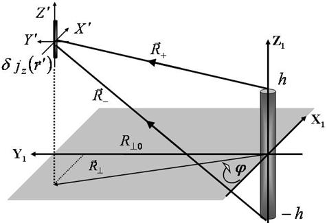
We
have come up closely to our basic model of random electric dipole source inside
a biological object oriented parallel to single (Fig. 3) or coupled (Fig. 1)
tuned linear wire antennas. In this model only the random electric field ![]() created by random electric current
created by random electric current ![]() is taken into account. We think the last
random electric current as being confined inside a thin and finite cylindrical
region, which is extended in limits
is taken into account. We think the last
random electric current as being confined inside a thin and finite cylindrical
region, which is extended in limits ![]() along the
along the ![]() -axes and defined by a vector
-axes and defined by a vector ![]() in the
in the ![]() - plane
as, e.g., in the case of the single vibrator- dipole antenna (Fig.3). Integrating
the random electric volume current density variation
- plane
as, e.g., in the case of the single vibrator- dipole antenna (Fig.3). Integrating
the random electric volume current density variation ![]() over
the cylindrical region cross- section leads to a total random current variation
over
the cylindrical region cross- section leads to a total random current variation
![]() in chosen cross-section, with a
longitudinal correlation function spectral density giving by
in chosen cross-section, with a
longitudinal correlation function spectral density giving by

Here ![]() is a volume of the random electric dipole
source.
is a volume of the random electric dipole
source.
One started actually to consider
a problem of exciting single receiving linear wire antenna by thermal radiation
from local temperature inhomogeneity. In the framework of the introduced random
electric dipole source model, the ![]() - component
- component ![]() of the incident random electric field
along single vibrator- dipole antenna (Fig. 3) is given according to Eqs. (11)
and (56) by relation
of the incident random electric field
along single vibrator- dipole antenna (Fig. 3) is given according to Eqs. (11)
and (56) by relation

where a
Green function ![]() is obtained from
is obtained from ![]() defined after Eq.(34) by replacing
defined after Eq.(34) by replacing ![]() to
to ![]() and
and ![]() to
to ![]() . The
incident random electric field in Eq.(58) excites along single tuned vibrator-
dipole receiving antenna a current distribution with random amplitude
. The
incident random electric field in Eq.(58) excites along single tuned vibrator-
dipole receiving antenna a current distribution with random amplitude ![]() given by Eq.(37), with replacing
given by Eq.(37), with replacing ![]() to
to ![]() in the
RHS integrand. Thus one gets
in the
RHS integrand. Thus one gets

Applying to
the RHS of this equation the integration part by part with respect to variable ![]() , similarly with integral in Eq. (43),
gives
, similarly with integral in Eq. (43),
gives
For the
case of tuned vibrator –dipole of length ![]() equal
to odd whole number
equal
to odd whole number ![]() of half wavelengths Eq. (60) is
transformed as
of half wavelengths Eq. (60) is
transformed as

where ![]() are defined by
are defined by ![]() (see
Fig.4). According to obtained equation the two spherical waves are propagated
from a point
(see
Fig.4). According to obtained equation the two spherical waves are propagated
from a point ![]() of random electric dipole source towards
receiving vibrator-dipole ends. Bearing in mind the reciprocity between receiving
and transmitting antennas one can say also that two spherical waves are
propagated from vibrator- dipole ends towards the random electric dipole source
and interfere on the source area. Eqs. (57) and (61) enable us to write out for
the fluctuations’ spectral density
of random electric dipole source towards
receiving vibrator-dipole ends. Bearing in mind the reciprocity between receiving
and transmitting antennas one can say also that two spherical waves are
propagated from vibrator- dipole ends towards the random electric dipole source
and interfere on the source area. Eqs. (57) and (61) enable us to write out for
the fluctuations’ spectral density ![]() of current
distribution along receiving antenna amplitude caused by random electric dipole
source thermal radiation a following equality
of current
distribution along receiving antenna amplitude caused by random electric dipole
source thermal radiation a following equality

|
|
|
|
|
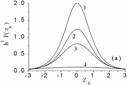
Figure 4. (a) The normalized interference
function versus normalized height
|
A
function ![]() in the RHS of this equality has a form of
integral
in the RHS of this equality has a form of
integral

where
integrand ![]() is defined by
is defined by
with ![]() . Similarly to optics [36] the definitions
in Eqs.(63) and (64) can be called the single linear wire receiving antenna interference
functions for the cases of finite extended and point random electric dipole
source, respectively.
. Similarly to optics [36] the definitions
in Eqs.(63) and (64) can be called the single linear wire receiving antenna interference
functions for the cases of finite extended and point random electric dipole
source, respectively.
The spatial integral averaging in the RHS of Eq. (63) along random electric dipole source extension we perform using an approximate formula
 (65)
(65)
where a function
![]() . This formula is derived by writing
. This formula is derived by writing ![]() and approximate bringing the denominator
and approximate bringing the denominator ![]() outside the integral in the middle point
outside the integral in the middle point![]() . Actually we needs spatial averaging the
fast varying cosine term of
. Actually we needs spatial averaging the
fast varying cosine term of ![]() only that gives for
only that gives for ![]() an expression
an expression

As one
sees the interference function ![]() for finite extended random
electric dipole source is different from such interference function
for finite extended random
electric dipole source is different from such interference function ![]() for point source on a
for point source on a ![]() -factor that defines a spatial coherence
degree of extended random electric dipole source.
-factor that defines a spatial coherence
degree of extended random electric dipole source.
Our next task consists in study
the interference function ![]() extreme properties
depending on random electric dipole source extension and
extreme properties
depending on random electric dipole source extension and ![]() position defined by mentioned above
coordinate
position defined by mentioned above
coordinate ![]() and vector
and vector ![]() . In
this case the coordinate
. In
this case the coordinate ![]() gives height of random
electric dipole source centre above (
gives height of random
electric dipole source centre above (![]() ) or under (
) or under (![]() ) the single linear wire antenna
) the single linear wire antenna ![]() - plane (Fig. 3) while the vector
- plane (Fig. 3) while the vector ![]() characterizes
characterizes ![]() position
of random electric dipole source centre projection on the
position
of random electric dipole source centre projection on the ![]() -plane that can be characterized also by
the vector
-plane that can be characterized also by
the vector ![]() length
length ![]() and
its azimuth angle
and
its azimuth angle ![]() (see Fig. 3). The minimum value
(see Fig. 3). The minimum value
![]() of the vector
of the vector ![]() length
corresponds to the azimuth angle
length
corresponds to the azimuth angle ![]() and gives us the real
depth of random electric dipole source centre, with
and gives us the real
depth of random electric dipole source centre, with ![]() being
a seeming depth of this source centre. Henceforth the aim of the single
receiving antenna scanning along biological object boundary surface
being
a seeming depth of this source centre. Henceforth the aim of the single
receiving antenna scanning along biological object boundary surface ![]() consists to get the random electric
dipole source centre inside the
consists to get the random electric
dipole source centre inside the ![]() -plane, first, and to
define the source centre real depth by, e.g., placing this centre on the
-plane, first, and to
define the source centre real depth by, e.g., placing this centre on the ![]() - axes, second. We intend to show that
interference function
- axes, second. We intend to show that
interference function ![]() extreme properties can be a
physical base to realize such kind of single receiving antenna scanning
strategy.
extreme properties can be a
physical base to realize such kind of single receiving antenna scanning
strategy.
The
interference function ![]() has extreme value – maximum at
has extreme value – maximum at ![]() , at last. One can verify this statement
easily in the simple case of point random electric dipole source, with
neglecting effect of absorption when interference function
, at last. One can verify this statement
easily in the simple case of point random electric dipole source, with
neglecting effect of absorption when interference function ![]() has for small
has for small ![]() the
Taylor expansion
the
Taylor expansion

Here ![]() is maximum value of
is maximum value of ![]() , with
, with ![]() being
equal to
being
equal to ![]() at
at ![]() The
quantity
The
quantity ![]() is half width at half maximum (HWHM) of
the Taylor expansion in Eq.
(67). A constant
is half width at half maximum (HWHM) of
the Taylor expansion in Eq.
(67). A constant ![]() in the RHS of the second Eq.(67)
in the RHS of the second Eq.(67)
is
defined as ![]() for the half wavelength vibrator antenna.
for the half wavelength vibrator antenna.
Eq.(67) shows that HWHM of
interference function ![]() can be used to determine the seeming
depth
can be used to determine the seeming
depth ![]() of random electric dipole point source. Because
the HWHM is experimentally measured quantity we study next the interference
function
of random electric dipole point source. Because
the HWHM is experimentally measured quantity we study next the interference
function ![]() extreme points and their HWHM in details,
with taking into account effects of absorption and random electric dipole source
extension.
extreme points and their HWHM in details,
with taking into account effects of absorption and random electric dipole source
extension.
Fig.4(a) presents calculated by
Eq.(64) dependence of the normalized interference function ![]() on normalized height
on normalized height ![]() of random electric dipole point source at
a set of the point source normalized seeming depths
of random electric dipole point source at
a set of the point source normalized seeming depths ![]() ranged
from 1 up to 6 when the curves have only one peak and absorption is neglected. From
this calculated curves we take HWHM and plot HWHM against the known normalized
seeming depth
ranged
from 1 up to 6 when the curves have only one peak and absorption is neglected. From
this calculated curves we take HWHM and plot HWHM against the known normalized
seeming depth ![]() (Fig.4(b), curve 1). The curve 2 in the Fig.4(b) plots HWHW according to
the Taylor expansion in Eq.
(67) that is the quantity
(Fig.4(b), curve 1). The curve 2 in the Fig.4(b) plots HWHW according to
the Taylor expansion in Eq.
(67) that is the quantity ![]() . The Fig. 4 shows that
HWHM of interference function growths monotonously with growing the random
electric dipole point source seeming depth when effect of biological object
absorption is neglected. The curve 2 in Fig.4(b) predicts substantially smaller value for HWHM at given
. The Fig. 4 shows that
HWHM of interference function growths monotonously with growing the random
electric dipole point source seeming depth when effect of biological object
absorption is neglected. The curve 2 in Fig.4(b) predicts substantially smaller value for HWHM at given ![]() compared with the curve 1 in Fig.4(b) since the Taylor expansion
dealing with only the peak top of the curves in the Fig.5(a). In Fig. 5 we
repeat the curve 1 from Fig.4(b) and test the role of absorption in the case of
point source. The absorption is measured in the units of
compared with the curve 1 in Fig.4(b) since the Taylor expansion
dealing with only the peak top of the curves in the Fig.5(a). In Fig. 5 we
repeat the curve 1 from Fig.4(b) and test the role of absorption in the case of
point source. The absorption is measured in the units of ![]() where n = 1, 2, and 3. The units of
absorption measurement are chosen, with taking into account that for tuned
vibrator-dipole
where n = 1, 2, and 3. The units of
absorption measurement are chosen, with taking into account that for tuned
vibrator-dipole ![]() and for the human head brain
and for the human head brain ![]() , according to Introduction.
, according to Introduction.
|
|
|
Figure 5. The normalized seeming depth
|
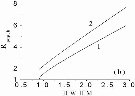
Fig.5 shows
that the more absorption is the less HWHM corresponds to the given point source
seeming depth. In another words, the maximum peak of interference function ![]() at
at ![]() becomes
narrower with growing absorption.
becomes
narrower with growing absorption.
|
|
|
|
|
Figure 6. The normalized seeming depth
|
Figs.6(a,b) depict HWHM of interference
function against the normalized seeming depth ![]() at a
set of random electric dipole source normalized extensions
at a
set of random electric dipole source normalized extensions ![]() , with
neglecting absorption, Fig.6(a), and accounting absorption, Fig.6(b). It is
seen from the panels (a) and (b) of Fig.6 that the absorption leads only to an
increase in the slope angle of a “bundle” of the curves with respect to the
HWHM axis. From the other hand, comparison of Fig.5 and Figs.6 demonstrates that
absorption and source extension make change in different manner the HWHM
dependence on source centre seeming depth. As one can note, the maximum peak of
interference function
, with
neglecting absorption, Fig.6(a), and accounting absorption, Fig.6(b). It is
seen from the panels (a) and (b) of Fig.6 that the absorption leads only to an
increase in the slope angle of a “bundle” of the curves with respect to the
HWHM axis. From the other hand, comparison of Fig.5 and Figs.6 demonstrates that
absorption and source extension make change in different manner the HWHM
dependence on source centre seeming depth. As one can note, the maximum peak of
interference function ![]() at
at ![]() becomes
wider with growing the source extension in both cases of neglecting and
accounting absorption. In addition to noted the effects of absorption and source
extension are more sensitive for relatively big and small source centre seeming
depths, respectively. Fig.5 curves allow one as to determine the point source
seeming depth at given absorption as Fig.6(b) curves permit one to get a source
centre seeming depth, with knowing biological object absorption and the source
extension. If in the last case the source extension is known approximately with
some accuracy the source centre seeming depth is obtained also approximately
with corresponding accuracy.
becomes
wider with growing the source extension in both cases of neglecting and
accounting absorption. In addition to noted the effects of absorption and source
extension are more sensitive for relatively big and small source centre seeming
depths, respectively. Fig.5 curves allow one as to determine the point source
seeming depth at given absorption as Fig.6(b) curves permit one to get a source
centre seeming depth, with knowing biological object absorption and the source
extension. If in the last case the source extension is known approximately with
some accuracy the source centre seeming depth is obtained also approximately
with corresponding accuracy.
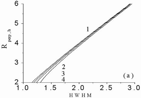
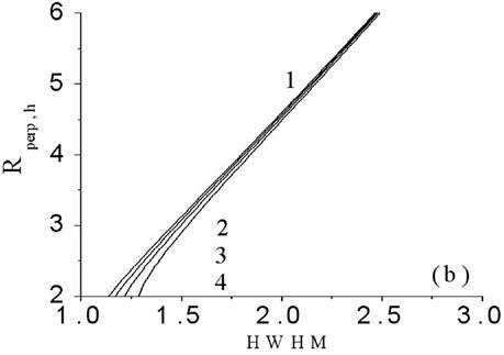
Having described Fig.4(a), we mentioned that the normalized interference function curves have only peak when source normalized seeming depth ranged from 1 up to 6 and absorption is neglected. Fig.7(a,b) shows that for smaller values of source normalized seeming depth the normalized interference function curves can have several peaks, with possibility for side peaks being not less the central peak (Fig.7, curve 4 has three equal peaks). The side peaks may be studied in manner similar to the central peak consideration. Nevertheless we will not study side peaks here.
Figs.4, 5, and 6 show that one
can actually get the random electric dipole source centre inside the ![]() -plane of a single receiving linear wire
antenna (Fig.3), via scanning this antenna along the
-plane of a single receiving linear wire
antenna (Fig.3), via scanning this antenna along the ![]() -
axis on the biological object boundary surface
-
axis on the biological object boundary surface ![]() = 0
and defining the HWHM of antenna interference function
= 0
and defining the HWHM of antenna interference function ![]() maximum
at
maximum
at ![]() = 0. As this takes place we obtain the
source centre seeming depth
= 0. As this takes place we obtain the
source centre seeming depth ![]() , with knowing the object absorption and
source extension. Now we intend to define the real depth
, with knowing the object absorption and
source extension. Now we intend to define the real depth ![]() of the source centre in the centre of
of the source centre in the centre of ![]() position inside the
position inside the ![]() -plane, via antenna scanning along the
-plane, via antenna scanning along the ![]() -axis on biological object boundary
surface.
-axis on biological object boundary
surface.
|
|
|
|
|
Figure 7. The normalized interference function
versus normalized height of random electric dipole point source with
neglecting object absorption at different relatively small values of the
point source normalized seeming depths: (a)
|
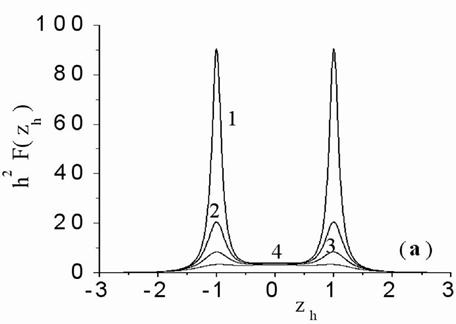
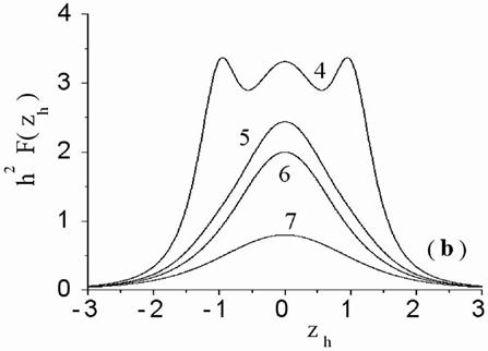
|
Figure
8. Schematic showing of the
upper half space of the
|
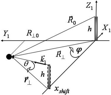
|
|
|
Figure 9. Dependence of the normalized interference function on a shift of
the
|
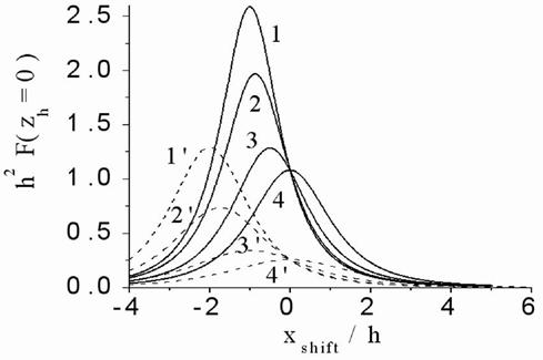
Fig.9 depicts schematically scanning
the random electric dipole extended source with centre on the ![]() -plane by shifting the single receiving
linear wire antenna along
-plane by shifting the single receiving
linear wire antenna along ![]() -axis to position with
coordinate
-axis to position with
coordinate ![]() The interference function
The interference function ![]() of the shifted single antenna is obtained
from Eq.(66) by setting
of the shifted single antenna is obtained
from Eq.(66) by setting ![]() and has a form
and has a form

with ![]() where
where![]() . The
quantity
. The
quantity ![]() is function of shifted antenna position
and given (Fig. 8) by relation
is function of shifted antenna position
and given (Fig. 8) by relation
![]() (69)
(69)
where ![]() ,
, ![]() is
projection of vector
is
projection of vector ![]() on the
on the ![]() -axis.
All quantities in Eqs.(68) and (69), having dimension of length, are normalized
to antenna half length
-axis.
All quantities in Eqs.(68) and (69), having dimension of length, are normalized
to antenna half length ![]() .
.
The interference function of the
shifted single antenna in Eq.(68) has evidently maximum at ![]() where the scanning antenna is brought in nearest
position to the random electric dipole extended source, with distant
where the scanning antenna is brought in nearest
position to the random electric dipole extended source, with distant ![]() between source centre and antenna centre becoming
equal to the real depth
between source centre and antenna centre becoming
equal to the real depth ![]() of the source centre.
The two quantities
of the source centre.
The two quantities ![]() and
and ![]() are
connected between them by relation
are
connected between them by relation ![]() . Therefore one can
get the real depth of the source centre
. Therefore one can
get the real depth of the source centre ![]() ,
provided one knows from scanning experiment the antenna position
,
provided one knows from scanning experiment the antenna position ![]() where antenna interference function has
maximum. We have also possibility to determine the real depth of the source
centre by study the maximum peak of interference function in Eq.(68). The Taylor expansion for small values of
where antenna interference function has
maximum. We have also possibility to determine the real depth of the source
centre by study the maximum peak of interference function in Eq.(68). The Taylor expansion for small values of ![]() gives a representation similar to one in
Eq.(67) and written as
gives a representation similar to one in
Eq.(67) and written as
 (70)
(70)
Here ![]() is maximum value of
is maximum value of ![]() . The quantity
. The quantity ![]() is
HWHM of the Taylor expansion in
Eq. (70) defined by
is
HWHM of the Taylor expansion in
Eq. (70) defined by
 (71)
(71)
where quantity
![]() and function
and function ![]() is
defined according to
is
defined according to
 (72)
(72)
Eq. (71)
shows that the HWHM ![]() is related to the real depth of
the source centre
is related to the real depth of
the source centre ![]() directly and becomes smaller
with absorption growing. Bearing in mind an asymptotics
directly and becomes smaller
with absorption growing. Bearing in mind an asymptotics ![]() as
as
![]() , one can conclude also that the HWHM
, one can conclude also that the HWHM ![]() increases with taking into account a
small extension of the source.
increases with taking into account a
small extension of the source.
|
|
|
Figure 10. Dependence of HWHM of interference function Eq. (68) on the azimuth
angle
|
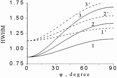
Fig.9 presents the normalized
interference function from Eq.(68) versus to normalized shift ![]() of scanning along
of scanning along ![]() -axis
antenna,. with no absorption taking into account. Fig.9 shows that normalized interference
function from Eq.(68) shift towards negative
-axis
antenna,. with no absorption taking into account. Fig.9 shows that normalized interference
function from Eq.(68) shift towards negative ![]() -axis
direction with decreasing azimuth angle
-axis
direction with decreasing azimuth angle ![]() according
to above position of the normalized interference function maximum. Meanwhile the
normalized interference function becomes wider with growing the azimuth angle
according
to above position of the normalized interference function maximum. Meanwhile the
normalized interference function becomes wider with growing the azimuth angle ![]() , that calls for growing the real depth of
the source centre, and with growing the source extension also. Fig.10 presents the
HWHM of normalized interference function from Eq.(68) versus to the varied azimuth
angle
, that calls for growing the real depth of
the source centre, and with growing the source extension also. Fig.10 presents the
HWHM of normalized interference function from Eq.(68) versus to the varied azimuth
angle ![]() at fixed the normalized seeming depth but
for a set of source extension, with no absorption taking into account. Fig. 10
shows again that the normalized interference function becomes wider with growing
the source extension.
at fixed the normalized seeming depth but
for a set of source extension, with no absorption taking into account. Fig. 10
shows again that the normalized interference function becomes wider with growing
the source extension.
|
|
|
Figure
11. Dependence
of HWHM of interference function Eq.(68) on azimuth angle
|
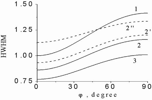
Fig. 11 generalizes content of Fig.10 on the subject to take into account the absorption, showing that the normalized interference function from Eq.(68) becomes narrower with growing absorption and wider with growing the source extension. Fig.12 presents the final dependence of normalized real depth of centre of random electric dipole extended source versus the HWHM of normalized interference function from Eq. (68), with taking into account absorption. The curves in Fig.12 show a competition between effects of absorption and source extension that make the HWHM smaller and bigger, respectively. As a result of such competition it is seen a crossing, in particular, of two curves (1 and 2”) in Fig. 12.
|
|
|
Figure
12. Dependence
of the normalized depth of the source position on the HWHM (Fig.11) at
|
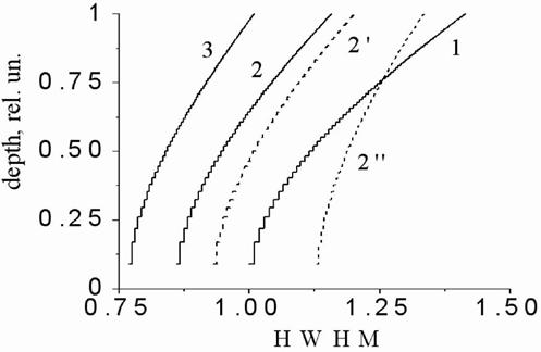
Before
going above to study the maximum peak of interference
function in Eq.(68), we had mentioned that one can get the real depth of the
source centre if one knows from scanning experiment the antenna position on ![]() -axis where antenna interference function
has maximum. In this case the three points’ set consisting of antenna centre
origin position, the just mentioned shifted antenna position and the source
centre position inside the
-axis where antenna interference function
has maximum. In this case the three points’ set consisting of antenna centre
origin position, the just mentioned shifted antenna position and the source
centre position inside the ![]() -plane (see
Fig.8) form
a rectangular triangle. Let us note
in order to generalize such kind forming a triangle that one can consider two positions
of two single antennas 1 and 2 centers along
-plane (see
Fig.8) form
a rectangular triangle. Let us note
in order to generalize such kind forming a triangle that one can consider two positions
of two single antennas 1 and 2 centers along ![]() -axis
of the
-axis
of the ![]() coordinate system (Fig. 13) when a
many-side triangle is formed inside the
coordinate system (Fig. 13) when a
many-side triangle is formed inside the ![]() -plane
by centers of these two antennas and random electric dipole source centre
projection on the
-plane
by centers of these two antennas and random electric dipole source centre
projection on the ![]() -plane. The lengths
-plane. The lengths ![]() and
and ![]() of
formed triangle two sides can be determined separately via scanning the antennas
1 and 2 along
of
formed triangle two sides can be determined separately via scanning the antennas
1 and 2 along ![]() - axis on biological object
boundary surface
- axis on biological object
boundary surface ![]() and defining the HWHM of these
antennas’ interference functions
and defining the HWHM of these
antennas’ interference functions ![]() and
and ![]() maximums at
maximums at ![]() , in
accordance with described study the interference function in Eq.(66). After
that one can determine the real depth
, in
accordance with described study the interference function in Eq.(66). After
that one can determine the real depth ![]() of random
electric dipole source centre by resolving the triangle , with knowing its two
mentioned sides as two seeming depths of source centre from two antennas
centers and knowing distant between antennas. A symmetrical position of random
electric dipole source relatively antennas, which transforms the above
many-side triangle into isosceles one, is especially interesting for the case
when effects of antennas’ coupling are taking into account. This case of two
coupled tuned receiving linear wire antennas’ exciting by the random electric
dipole source is our next task.
of random
electric dipole source centre by resolving the triangle , with knowing its two
mentioned sides as two seeming depths of source centre from two antennas
centers and knowing distant between antennas. A symmetrical position of random
electric dipole source relatively antennas, which transforms the above
many-side triangle into isosceles one, is especially interesting for the case
when effects of antennas’ coupling are taking into account. This case of two
coupled tuned receiving linear wire antennas’ exciting by the random electric
dipole source is our next task.
|
Figure 13. Schematic showing of two coupled antennas in thermal radiation field of local temperature inhomogeneity.
|
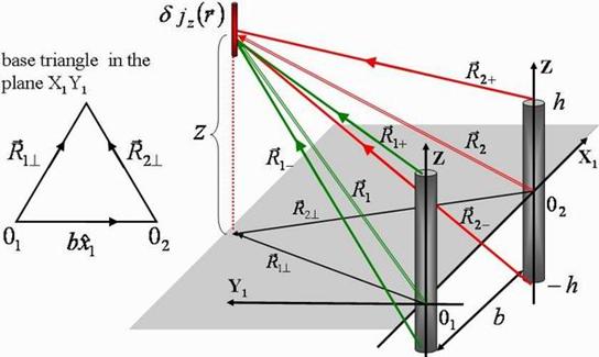
In the framework of using random
electric dipole source model the ![]() - component
- component ![]() of the incident random electric field
along as coupled vibrator-dipole antenna 1 in Fig. 13 is given as along single
vibrator-dipole antenna in Fig.3 by Eq.(58). Analogous expression for
of the incident random electric field
along as coupled vibrator-dipole antenna 1 in Fig. 13 is given as along single
vibrator-dipole antenna in Fig.3 by Eq.(58). Analogous expression for ![]() - component
- component ![]() of the
incident random electric field along coupled vibrator-dipole antenna 2 in Fig. 13 is obtained from Eq.(58) by
replacing
of the
incident random electric field along coupled vibrator-dipole antenna 2 in Fig. 13 is obtained from Eq.(58) by
replacing ![]() to
to ![]() . The
incident random electric fields
. The
incident random electric fields ![]() and
and ![]() excite along two coupled antennas some
current distributions with random amplitudes
excite along two coupled antennas some
current distributions with random amplitudes ![]() and
and ![]() given by Eqs.(41) and (42), respectively,
with replacing
given by Eqs.(41) and (42), respectively,
with replacing ![]() to
to ![]() and
and ![]() to
to ![]() in the
RHS integrands. Writing now equations similar to Eqs.(59) and (60) and supposing
the tuned vibrator-dipoles to be of length equal to add whole number of half
wavelengths lead us to generalization of Eq.(61) in the form
in the
RHS integrands. Writing now equations similar to Eqs.(59) and (60) and supposing
the tuned vibrator-dipoles to be of length equal to add whole number of half
wavelengths lead us to generalization of Eq.(61) in the form
 (73)
(73)
and
 (74)
(74)
Here sums
are taken over index ![]() two values
two values ![]() , with distances
, with distances ![]() and
and
![]() being defined similar to the case of
single antenna in Eq.(61) and related to antennas 1 and 2, respectively, in
Fig. 13. According to Eqs.(73) and (74) the two spherical waves are propagated
from a point
being defined similar to the case of
single antenna in Eq.(61) and related to antennas 1 and 2, respectively, in
Fig. 13. According to Eqs.(73) and (74) the two spherical waves are propagated
from a point ![]() of random electric dipole source towards
receiving vibrator-dipole 1 ends as well as two another spherical waves are
propagated from the same point of source towards receiving vibrator-dipole 2
ends. Bearing in mind the reciprocity between receiving and transmitting
antennas one can say also that four spherical waves are propagated from
vibrator- dipoles 1 and 2 ends towards the random electric dipole source and
interfere on the source area. Eqs.(57) jointly with Eqs.(73) and (74) enables
us to get for the fluctuations’ spectral densities
of random electric dipole source towards
receiving vibrator-dipole 1 ends as well as two another spherical waves are
propagated from the same point of source towards receiving vibrator-dipole 2
ends. Bearing in mind the reciprocity between receiving and transmitting
antennas one can say also that four spherical waves are propagated from
vibrator- dipoles 1 and 2 ends towards the random electric dipole source and
interfere on the source area. Eqs.(57) jointly with Eqs.(73) and (74) enables
us to get for the fluctuations’ spectral densities  of
current distributions’ along coupled receiving antennas 1 and 2 amplitudes caused
by random electric dipole source thermal radiation the following equalities
of
current distributions’ along coupled receiving antennas 1 and 2 amplitudes caused
by random electric dipole source thermal radiation the following equalities

which
generalize Eq.(62) written for a single antenna. Functions ![]() in the RHS of these equalities, with
indices
in the RHS of these equalities, with
indices ![]() related to coupled antennas 1 and 2, have
form of integral averaging along random electric dipole source extension in
Eq.(63), with integrands
related to coupled antennas 1 and 2, have
form of integral averaging along random electric dipole source extension in
Eq.(63), with integrands ![]() being presented as
being presented as
and
Functions
![]() here coincides in physical sense with
interference functions for point random electric dipole source exciting a
single antenna 1 or 2 and are defined accordingly to Eq.(64) by
here coincides in physical sense with
interference functions for point random electric dipole source exciting a
single antenna 1 or 2 and are defined accordingly to Eq.(64) by
where ![]() . While the functions in Eq.(78) we call the
auto-interference functions of single antennas 1 and 2, the functions
. While the functions in Eq.(78) we call the
auto-interference functions of single antennas 1 and 2, the functions ![]() and
and ![]() need
being called the cross-interference functions of coupled antennas because the
last two functions take into account interference between a couple of spherical
waves (see Fig. 13), one of which propagates from the point of random electric
dipole source towards a receiving vibrator-dipole 1 end and another propagates to
a receiving vibrator-dipole 2 end, as it is confirmed by equations
need
being called the cross-interference functions of coupled antennas because the
last two functions take into account interference between a couple of spherical
waves (see Fig. 13), one of which propagates from the point of random electric
dipole source towards a receiving vibrator-dipole 1 end and another propagates to
a receiving vibrator-dipole 2 end, as it is confirmed by equations
![]() (78)
(78)
and ![]() where
where ![]() is
phase of the coupling factor
is
phase of the coupling factor ![]() defined by
defined by ![]() . The sum in the RHS of Eq.(78) is taken over
both indices
. The sum in the RHS of Eq.(78) is taken over
both indices ![]() and
and ![]() two
values
two
values ![]() , with including four terms. The written
equations for the cross- interference functions of antennas include an addition
shift
, with including four terms. The written
equations for the cross- interference functions of antennas include an addition
shift ![]() caused by antennas coupling side by side
with phase shift
caused by antennas coupling side by side
with phase shift ![]() equal to paths differences of
two spherical waves in the biological object medium.
equal to paths differences of
two spherical waves in the biological object medium.
Consider
dependence of antennas interference functions ![]() ,
defined in Eqs.(76) and (77) for the case of point random electric dipole
source, on the antennas coupling factor
,
defined in Eqs.(76) and (77) for the case of point random electric dipole
source, on the antennas coupling factor ![]() . We
see this dependence in a simple form of scaling factors
. We
see this dependence in a simple form of scaling factors ![]() and
and
![]() as well as in a complicate form of the
addition phase shift in expressions for the cross-interference functions of
coupled antennas. Nevertheless the complicate phase shift comes into
as well as in a complicate form of the
addition phase shift in expressions for the cross-interference functions of
coupled antennas. Nevertheless the complicate phase shift comes into ![]() and
and ![]() with
opposite signs and hence transforms into a scale factor in the sum of these cross-interference
functions
with
opposite signs and hence transforms into a scale factor in the sum of these cross-interference
functions
![]() (79)
(79)
Summing next Eqs.(76) and (77), with accounting Eq.(79), gives
 (80)
(80)
Summing
at last the basic Eqs. (75) defined the fluctuations’ spectral densities and reminding definition of functions ![]() give us
give us
 (81)
(81)
with
 (82)
(82)
The
obtained three Eqs.(80), (81) and (82) show that sum of the fluctuations’
spectral densities of current distributions’ along coupled receiving antennas 1
and 2 amplitudes caused by random electric dipole source thermal radiation has
dependence on antennas coupling factor ![]() in a simple
form of scaling factors
in a simple
form of scaling factors ![]() and
and ![]() only.
only.
Although
the RHS of Eq.(81) has a simple dependence on antennas coupling factor, the RHS
of Eq. (80) leaves some difficult for study via complicate structure of four
term sum, with each term describing interference of a waves’ couple propagated
from a point source towards different antennas’ ends. Therefore we return to
general Eq.(78) for the cross-interference function of coupled antennas and
consider a mentioned above special case of symmetrical position of random
electric dipole source relatively antennas (Fig. 13) when a many-side triangle, formed
inside the ![]() -plane by centers of antennas and random
electric dipole source centre projection on the
-plane by centers of antennas and random
electric dipole source centre projection on the ![]() -plane,
becomes isosceles one. In this case of source symmetrical position we have
relations
-plane,
becomes isosceles one. In this case of source symmetrical position we have
relations ![]() , with index
, with index ![]() , that
simplifies Eq.(78) immediately as
, that
simplifies Eq.(78) immediately as
![]() (83)
(83)
where ![]() and
and ![]() is
given by Eq. (64). The final physically transparent result consists in
equations
is
given by Eq. (64). The final physically transparent result consists in
equations
 (84)
(84)
where  is presented in Eq.(62). Thus in the
special case of source symmetrical position relatively antennas the both cross-interference
functions of coupled antennas become equal to auto- interference function of
single antenna accurate to scaling factor
is presented in Eq.(62). Thus in the
special case of source symmetrical position relatively antennas the both cross-interference
functions of coupled antennas become equal to auto- interference function of
single antenna accurate to scaling factor ![]() as
well as the fluctuations’ spectral densities of current distributions’ along
coupled receiving antennas 1 and 2 amplitudes become equal to fluctuations’
spectral densities of current distributions’ along single antennas accurate to
scaling factor
as
well as the fluctuations’ spectral densities of current distributions’ along
coupled receiving antennas 1 and 2 amplitudes become equal to fluctuations’
spectral densities of current distributions’ along single antennas accurate to
scaling factor ![]() . Ultimately one can reduce the
scanning problem of random electric dipole source via two coupled tuned
receiving linear wire antennas to considered already such scanning problem via
a single antenna, provided one is able to place the scanning source into
symmetrical position relatively antennas and move the antennas 1 and 2
together, not separately, along
. Ultimately one can reduce the
scanning problem of random electric dipole source via two coupled tuned
receiving linear wire antennas to considered already such scanning problem via
a single antenna, provided one is able to place the scanning source into
symmetrical position relatively antennas and move the antennas 1 and 2
together, not separately, along ![]() -axes on biological boundary
surface
-axes on biological boundary
surface ![]() (Fig. 13).
(Fig. 13).
Conclusions
Theory of electromagnetic wave multiple scattering by ensemble of dielectric and conductive bodies has been applied to study coupled receiving antennas. A basic exact system of Fredholm’s second kind integral equations for electric currents excited inside antennas is derived and written in terms of the electric field tensor T-scattering operator of a single antenna, the electric field retarded Green tensor function of a background and the incident on antennas electric field. In this equations’ system an antenna is a body with given complex dielectric permittivity on some frequency, and electric current excited inside the antenna means sum of volume conducting and displacement electric currents. The background medium can be inhomogeneous one with some complex dielectric permittivity. The kernels of derived integral equations’ system are not singular for the case of no overlapping antennas, although the background electric field Green tensor function is singular in the origin. Such kind of three - dimensional singularity has been met really at study the wave integral equation for electric field inside single antenna in the homogeneous background, by verifying consistence this integral equation with boundary conditions on the antenna surface. As was demonstrated, one has to take into account two sorts of the homogeneous background electric field Green tensor function strong singularity: (i) electric field Green tensor function decomposition into a delta Dirac function term and principal part, and (ii) rule to bring out the second derivative outside the three-dimensional singular integral.
The derived integral equations’ system for electric currents excited inside coupled antennas has been applied to study near field coherent effects caused by thermal microwave radiation incident electric field distribution along single or two coupled linear wire perfectly conducting receiving antennas in the form of thin vibrator- dipoles placed at heated biological object boundary surface and tuned to half wavelength in the object. After having been neglected wave interaction of antennas with biological object boundary surface and used asymptotic method of “big logarithm”, the T-scattering operator of single antenna in the form of tuned vibrator-dipole has become a separable wire T- scattering operator that lead to analytic evaluating the local total currents on two coupled receiving antennas and got a dimensionless antennas’ coupling factor. Effects of homogeneous and local inhomogeneous biological object temperature components on receiving antennas have been considered. Homogeneous temperature component was treated as source for equilibrium thermal radiation with standard form of incident on receiving antennas electric field spatial correlation function. This treatment led to a generalized Nyquist formula for currents’ fluctuations excited on coupled receiving vibrator- dipole antennas, with accounting the auto- correlation and cross- correlation functions of random electric field inside each antenna and on both antennas, respectively. More original results have been obtained at study effects of biological object temperature distribution local volume change in the model framework of random electric dipole source inside object absorption skin slab area, with dipole source being parallel to vibrator-dipole antennas parallel between themselves and placed on the object surface. In the case of single receiving vibrator-dipole antenna it was shown that two spherical waves are propagated from a point of random electric dipole source towards receiving vibrator-dipole ends. Bearing in mind the reciprocity between receiving and transmitting antennas one can say also that two spherical waves are propagated from vibrator- dipole ends towards the random electric dipole source and interfere on the source area. This physical interpretation led similarly with optics to single antenna auto-interference function. Extreme properties of single antenna auto-interference function depending on random electric dipole source extension and the source centre three-dimension position relatively receiving antenna on the biological object surface have been studied in details. It was shown, in particular, that the single antenna auto-interference function has maximum at source centre near antenna equatorial plane, with half width at half maximum (HWHM) becoming narrower and wider under biological object absorption and source extension growing, respectively. Ultimately a method of random electric dipole source scanning via single receiving vibrator- dipole antenna moving along the biological object surface was formulated. Two scanning most simple strategy was considered: (i) by defining via HWHM the two values of source centre seeming depth relatively two antenna positions with next evaluating the real depth of the source centre (many-side triangle strategy), and (ii) by getting a symmetrical position of source relatively two antenna positions that transforms the many-side triangle into a isosceles one (isosceles triangle strategy).
In the case of two coupled receiving vibrator-dipole antennas 1 and 2, as was shown two spherical waves are propagated from a point of random electric dipole source towards receiving vibrator-dipole 1 ends as well as two another spherical waves are propagated from the same point of source towards receiving vibrator-dipole 2 ends. Hence side by side with above single antennas 1 and 2 auto-interference functions, a cross-interference function of coupled antennas 1 and 2 has been introduced. The cross-interference function includes a complicate dependence on antennas coupling factor phase. Nevertheless, in the special case of source symmetrical position relatively antennas the cross-interference function of coupled antennas become equal to auto- interference function of single antenna, accurate to scaling factor equal to antennas coupling factor phase cosine. At the same time the fluctuations’ spectral densities of current distributions’ along coupled receiving antennas 1 and 2 amplitudes become equal to fluctuations’ spectral densities of current distributions’ along single antennas, accurate to scaling factor in the simple algebraic form of antennas coupling factor. Ultimately, the scanning problem of random electric dipole source via two coupled tuned receiving linear wire antennas has been reduced to such scanning problem via a single antenna, provided one is able to place the scanning source into symmetrical position relatively antennas and move the antennas 1 and 2 together, not separately, along biological object boundary surface.
Acknowledgments
This work was supported in part by Russian Foundation for Basic Research, Grant 09-02-00920-a, by the Russian Academy of Sciences project “ Passive multichannel human radio- and acusto-thermotomography in near zone” and “Investigations of new types of photonic crystals for development of optoelectronic elements of infocommunicationic nets”.
References
1. Godik E.E., Gulyev Yu.V. Functional imaging of the human body // IEEE Engineering in Medicine and Biology, 10, 21, 1991.
2. Reznik A.N. Quasistatic field of thermal radiation in theory of contact radiothermomatry // Izv. Vyssh. Uchebn. Zaved., Radiofiz, 34, 512, 1991.
3. Reznik A.N., Vaks V.L.,Yurasova N.V.Quasistationary field of thermal emission and near-field radiometry // Phys. Rev. E, 70, 056601-1, 2004.
4. Gaikovich K.P., Reznik A.N., Vaks V.L.,Yurasova N.V. New effect in near-field thermal emission // Phys. Rev. Lett, 88, 104302-1, 2002.
5. Anzimirov V.L., Arkhipova N.A., Pasechnik V.I., Yanovich A.V. Investigationtic of thermal excitation in human head brain core at functional tests by method of dynamic multichannel radiothermovision // Biomed. Radioelektron., 8, 22, 2000.
6. Rytov S.M. Theory of electric fluctuations and thermal radiation. Akad. Nauk SSSR, Moscow, 1953 [in Russian].
7. Landau L.D., Lifshitz E.M. Electrodynamics of continuous media. Gostechisdat, Moscow, 1957.
8. Cilin V.P.,Ruchadze A.A. Electromagnetic properties of plasma and plasma like bodies. Gostechisdat, Moscow, 1961.
9. Levin M.L., Rytov S.M. Theory of equilibrium thermal fluctuations in electrodidamics. Nauka, Moskow, 1967 [in Russian].
10. Rytov S.M., Kravtsov Yu.A., Tatarskii V.I. Principles of statistical radiophysics.Vol. 3. Wave propagation through random media. Springer, Berlin, 1989.
11. Honl H., Maue W., Westpfahl K. Theorie der beugung. Springer, Berlin, 1966.1961.
12. Goldberger M.L., Watson K.M. Collision theory. Wiley, New York, 1964.
13. Newton R.G., Scattering theory of waves and particles. McGraw-Hill, New York, 1966.
14. Frish V. Probabilistic methods in applied mathematics. Vol.1, edited by Bharucha-Reid. Academic, New York, 1968.
15. Barabanenkov Yu.N. Multiple scattering of waves by ensemble of particles and the radiative transport// Sov. Phys. Uspekhi, 18, 673, 1975.
16. Tsang L., Kong J.A. Multiple scattering of electromagnetic waves by random distributions of discrete scatterers with coherent potential and quantum mechanical formalism// J. Appl. Phys., 51, 3465, 1980.
17. Gulyaev Yu.V., Barabanenkov Yu.N., Barabanenkov M.Yu., Nikitov S.A. Optical theorem for electromagnetic field scattering by dielectric structures and energy emission from the evanescent wave //Phys. Rev.E, 72, 1, 2005.
18. Leontovich M.A, Levin M.L. To theory of oscillation excitation in vibrator antennas// Journ. Thechn. Phys. 14,481, 1944.
19. Hallen E.Theoretical investigation into the transmission and receiving qualities of antennae// Nova Acta Regiae Soc. Sci. Upsaliensis, Ser.IV, No. 4, 1-44, 1938.
20. Pocklington H.C. Electrical oscillation in wire// Cambridge Philos. Soc. Proc., 9, 324, 1897.
21. King R, Harrison C.W. Mutual and self- impedance for coupled antennas// J. Appl. Phys.15, 481, 1944.
22. King R. The theory o f N coupled parallel Antennas// J. Appl. Phys. 21, 94, 1950.
23. Markov G.T. Approximate calculation of mutual impedance for antennas// Radiotechnik. 3, 36, 1948.
24. Brillouin L. The Radiation Resistance of Resonant Transmission Line //Radioelectricite Sommaire , p.147, April, 1922.
25. Pistolkors A.A. The radiation resistance of antennas and antenna combinations// Proc. IRE, 17, 526,1929.
26. Bechmann R. On the calculation of radiation resistance of antennas and antenna combination// Proc. IRE, 19, 461,1931.
27. Stratton J.A. Electromagnetic theory. McGray-Hill, New York, 1941.
28. Foldy L.L. The multiple scattering of waves // Phys. Rev. 67, 107, 1945.
29. Lax M. MultiSpringerple scattering of waves// Rev. Mod. Phys. 23, 287, 1951.
30. Vasilyev E.N. Exitation of rotation bodies. Radio and Communiction, Moscow, 1987.
31. Van Bladen J. Some remarks on Green’s dyadic for infinite space// IRE Trans. Ant. And Prpop. AP-9, 563, 1961.
32. V.M. Finkelberg. Dielectric permittivity of mixtures// Journ. Techn.Phys. 34, 509, 1964.
33. Gelfand I.M., Shilov G.E. Gwnwlalized functions. Vol. 1: poreties and operators. Academic Press, Boston, 1964.
34. Mallet P., Guerin C.A., Sentenas A. Maxwell-Garnet mixing rule in the presence of multiple scattering: Derivation and accuracy// Phys. Rev. b, 72, 014205, 2005.
35. Mikhlin S.G., Prossdorf S. Singular integral operators. Springer, 1987.
36 Born M., E. Wolf E. Principles of optics. Pergamon Press, New York , 1964.
37. Balanis C.A. Antenna theory (analysis and design). A John Wiley&Sons, New Jersey, 2005.
38. Korn G.A., Korn T.M. Mathematical handbook (for scientists and engeneers). McGray-Hill, New York, 1961.
39. Nyquist H. Thermal agitation of conductors // Phys. Rev. 29, 614, 1927.