UDC 520.622
The simulating of image formation with subdiffraction resolution using one-dimensional experimental structure of scanning single aperture terahertz telescope
A. N. Vystavkin1, 3, S. E. Bankov1,3, M. E. Zhukovskij2,3, S. V. Podoljako2,3, O. V. Korjukin1,
Yu. N. Kazantsev1, A. G. Kovalenko1, E. A. Vystavkin1,3, A. S. Iliin1
1 V.A. Kotel’nikov Institute of Radioengineering and Electronics of RAS
2 M.V. Keldysh Institute of Applied Mathematics of RAS
3 LLC “Laboratory of Terahertz Radiometers”, the participant of Skolkovo Innovation
Center
The paper is received on December 1, 2015
Abstract. A method is proposed that allows to largely overcome the diffraction limit, as well as noise and other interferences in radio imaging devices (including ground and space telescopes) of millimeter, terahertz and far infrared ranges of the electromagnetic radiation in conformity with problems of reconstruction of images of the observing objects (the density distribution of sources). The spatial (angular) resolution and precision of the distributions of the observing sources are significantly higher in comparison with existing radio imaging devices of the specified ranges. This article describes the mathematical methods used to solve these problems. The article focuses on the simplest problem of the simulating of the image formation with a subdiffraction resolution using a one-dimensional experimental model of single aperture telescope. It is described the named experimental model and the corresponding experimental setup, the main components of which are the source of the electromagnetic radiation with a wavelength of ![]() mm on the basis of the backward wave tube, the telescope imitator based on two paired Teflon lenses, the radiation detector in the form of optic-acoustic receiver (Golay cell) and two precision coordinate tables with the electrical drive that moves the telescope imitator and the Golay cell. Due to the said moving the work of the telescope itself and the image being observed are imitated. The result of the modeling has revealed itself in the estimation of improvement of the spatial (angular) resolution of radio the imaging devices of the specified above ranges up to ~ 150 times.
mm on the basis of the backward wave tube, the telescope imitator based on two paired Teflon lenses, the radiation detector in the form of optic-acoustic receiver (Golay cell) and two precision coordinate tables with the electrical drive that moves the telescope imitator and the Golay cell. Due to the said moving the work of the telescope itself and the image being observed are imitated. The result of the modeling has revealed itself in the estimation of improvement of the spatial (angular) resolution of radio the imaging devices of the specified above ranges up to ~ 150 times.
Key words: radioastronomy and radio imaging devices of terahertz range of electromagnetic radiation, ground and space telescopes, methods of improving the characteristics, including the angular resolution, of telescopes and radio imaging devices.
Introduction.
The authors of the patent[1] have proposed the method permitting to largely overcome the diffraction limit as well as a noise and other interferences in radio imaging devices (including the ground and space telescopes) of millimeter, terahertz and far infrared ranges of the electromagnetic radiation in conformity with problems of the reconstruction of images of observed objects (the distribution of radiation sources density). The spatial (angular) resolution and sharpness of the getting distributions of sources are significantly higher in comparison with existing radio imaging devices of the specified ranges, to which the mentioned above method has not been applied. This means the single aperture radio imaging devices, and observed images means two-dimensional.
The distribution function of the radiation sources density is the solution of the integral equations of the first kind. The corresponding problems of finding the specified function are ill posed. The instability of ill-posed problems and the inaccurate information about the input data require the development of so-called regularizing algorithms[2]. The requirements for these algorithms increase when considering tasks, the exact solutions of which are functions with a complex structure (tears, corner points, etc.). To clarify the nature of the sought solution allows the use of prior information of various types[3].
The distribution function of the density of the sources is obviously a function with multi-scale structure due to the different brightness and contrast of images. This circumstance gives the rise to the presence of singularities in solution of problem (unsmoothed unknown function).
The traditional methods give “smoothing” of the solution in the vicinity of singularities of the unknown function (blurred solution), the greater, the greater inaccuracy of input data ![]() (this error is determined by the distortion of an optical system, error of the measuring system, as well as the presence of noise of different origin). The total distortion of the sought solution may be unacceptable even for moderate levels of error input data
(this error is determined by the distortion of an optical system, error of the measuring system, as well as the presence of noise of different origin). The total distortion of the sought solution may be unacceptable even for moderate levels of error input data ![]() .
.
However, in a wide range of applied problems there is a priority information about the solution, use which, when building the corresponding methods, can significantly improve the quality of approximate solutions[4, 5].
To do this, in the development of a regularization algorithm, it is necessary to use the methods of selection of approximations, ensuring convergence of the approximate solution to the exact one together with the derivative at the plots of the corresponding smoothness. Indeed, the visual nature of the change curve at a given point is defined by a coordinate and a direction of a tangent. Therefore, bringing on smooth areas, not only the decision itself, but also its derivative, it is possible to improve the quality of the approximations.
This article describes the simulation results of the proposed method of reconstruction of the distribution function of density of sources on the experimental one-dimensional model (the imitator) of single aperture telescope of millimeter range (λ ![]() 1.2 mm).
1.2 mm).
Methods of solving the considered problems
Consider the main features of the proposed algorithms and their differences from traditional methods of regularization.
Imagine the task in the operator form:
Here A is the integral operator of the 1st kind, f - the right side (the result of measurement), u - is the desired solution.
If the right part f is known not exactly, but with some error ![]() (
(![]() ,
, ![]() - the norm in functional space
- the norm in functional space![]() ), the approximate solutions
), the approximate solutions ![]() , some that
, some that ![]() can be arbitrarily hard to distinguish from each other when
can be arbitrarily hard to distinguish from each other when ![]() is arbitrarily small.
is arbitrarily small.
The vast majority of regularizing algorithms of solution of the problem (1), traditionally based in one form or another[2, 6] for minimization of the functional
At the same time ![]() - is the so-called stabilizer and
- is the so-called stabilizer and ![]() - regularization parameter. The stabilizer is introduced in order to ensure the stability of the resulting approximations to small changes of
- regularization parameter. The stabilizer is introduced in order to ensure the stability of the resulting approximations to small changes of![]() since solving the problem of minimizing the functional
since solving the problem of minimizing the functional ![]() does not possess the property of stability.
does not possess the property of stability.
In equation (2) one may see the cause of the above smoothing (blurring) of the solution. Such smoothing makes use of a completely continuous operator ![]() in functional
in functional ![]() .
.
To find the distribution function of sources in the present project it is proposed to use ideas of works[5-7]. The main difference is represented in these works, regarding algorithms and traditional methods, is that instead of (2) a variational problem of finding the minimum variation of the sought solution (or its derivatives) is introducing:
After this the ratio ![]() is considered as an additional condition, along with other conditions resulting from a priori information about the decision and recorded in the form of linear constraints on the desired solution.
is considered as an additional condition, along with other conditions resulting from a priori information about the decision and recorded in the form of linear constraints on the desired solution.
The variation of function characterizes the differentiability properties of this function, and the differential operator is unbounded and, therefore, may have a continuous inverse operator, that gives the opportunity to build sustainable solutions that preserve the properties of smoothness of the required function. The solution of the problem (3) does not require the introduction of "stabilizers" (it is possible to prove that the functionality ![]() is known as a "stabilizer"), and also allows to refuse from the concept of the regularization parameter
is known as a "stabilizer"), and also allows to refuse from the concept of the regularization parameter ![]() .
.
The proposed method of solution is as follows.
Consider the integral equation

The corresponding transformation of the density distribution of sources (unknown function ![]() ) to the measured value
) to the measured value ![]() (the image). In (4):
(the image). In (4): ![]() - the scope of
- the scope of ![]() ;
; ![]() - the scope of
- the scope of![]() .
.
Let the known measurement error ![]() due to the properties of measuring instruments, and diffraction effects, as well as "noise". Here
due to the properties of measuring instruments, and diffraction effects, as well as "noise". Here ![]() is marked the norm in the function space
is marked the norm in the function space ![]() .
.
As the desired function ![]() deals with the solution of the variational problem
deals with the solution of the variational problem
In the formula (5) ![]() is a variation
is a variation ![]() or its derivative. The problem (5) is solved under additional constraints on the desired function, which follow from a priori information about this feature. For example, the obvious is the requirement of nonnegativity of the solution
or its derivative. The problem (5) is solved under additional constraints on the desired function, which follow from a priori information about this feature. For example, the obvious is the requirement of nonnegativity of the solution ![]() .
.
The attraction of a priori information clarifies the nature of the required solution and in some cases, can significantly improve the accuracy of the approximations. Therefore, the more relevant methods is taken into account the available a priori information, the generally higher quality of the obtained approximate solutions.
Thus, the algorithm for the approximate solution of operator equation (4) is reduced to the solution of problem (5) under additional constraints relevant a priori information of various types and recorded in the form of linear conditions (inequalities) on the functionals of the desired solution.
In the numerical realization of the proposed method of reconstruction of distribution of density of sources conducted sampling two-dimensional fields ![]() and
and ![]() .
.
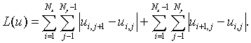
In the simplest case wherein (5) denotes the variation of function
minimized functionality in a discrete area
is written in the form:
The inequality ![]() makes sense limits and with the requirements of non-negativity of the sought solution (
makes sense limits and with the requirements of non-negativity of the sought solution (![]() ) as follows:
) as follows:
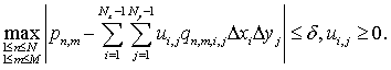
In the formula (7) the above symbols are introduced:
![]() ;
; ![]()
Thus, the solution of the original problem for the equation (4) is approximated by the solution of the discrete problem (6), (7).Note in concluding this section that, in practice, view the hardware features specific experiment (the kernel of equation (4)) is rarely known with sufficient degree of accuracy. Therefore, in the general case, the search for the required distribution of sources according to the observation is reduced to the solution of two problems:
1. Determining the response function of the system and
2. Proper reconstruction of the distribution function of the density of sources.
To address the first of the specified tasks approaches and algorithms are described in[7]. The ways of solving the problem (4) are based, as already mentioned, on the papers[5-7].
The formulation of the one-dimensional problem
The simplified one-dimensional diagram of the experiment is presented at Fig. 1.
Let the desired density of the distribution of radiation sources is ![]() . Let the center of telescope imitator is at the point
. Let the center of telescope imitator is at the point ![]() (Fig.1). The image
(Fig.1). The image ![]() of observed object is formed on the line of detectors s. The equation linking the density of sources and their images on the detector line, written in the form:
of observed object is formed on the line of detectors s. The equation linking the density of sources and their images on the detector line, written in the form:

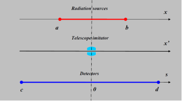
Fig.1. The simplified one-dimensional diagram of the experiment.
Thus, the problem of finding the function ![]() is reduced to the solution of the integral equation (8) of the first kind. Following the remarks at the end of the previous section, we first need to define a function
is reduced to the solution of the integral equation (8) of the first kind. Following the remarks at the end of the previous section, we first need to define a function ![]() . The kernel of integral operator
. The kernel of integral operator ![]() in equation (8) having the sense of the instrumental function of the experimental setup is determined as follows[7] :
in equation (8) having the sense of the instrumental function of the experimental setup is determined as follows[7] :

Formally, the relation (9) determines the response of the “optical” and measurement system (in our case – series (line) of detectors) (see ahead) to a point source of unit power (i.e.  ). The equality (9) indicates the method how to determine the kernel of the integral equation (8) being the hardware feature of the one-dimensional experiment. That is, in
order to build ![]() , one must measure the signal
, one must measure the signal ![]() at each point
at each point ![]() from the radiation delta-source at each point
from the radiation delta-source at each point ![]() .
.
It is important to note that the function ![]() is defined by the “optical” system, so and by measuring (recording) device.
is defined by the “optical” system, so and by measuring (recording) device.
For the numerical solution of equation (8) it is necessary to perform discretization of the problem. It is introducing two discrete grid: ![]() and grid
and grid ![]() . Using such discrete grids in some way approximated the density of sources
. Using such discrete grids in some way approximated the density of sources ![]() and the readings of the detectors
and the readings of the detectors ![]() and also the kernel
and also the kernel ![]() of equation (8).
of equation (8).
The function values ![]() at the nodal points of the two-dimensional area
at the nodal points of the two-dimensional area ![]() are obtaining by menace of the measuring the signal from a point source, located at the point
are obtaining by menace of the measuring the signal from a point source, located at the point ![]() by detector located at the point
by detector located at the point ![]() for all values j, n. The function values
for all values j, n. The function values ![]() at intermediate points of the region
at intermediate points of the region ![]() can be obtained, for example, using bilinear interpolation.
can be obtained, for example, using bilinear interpolation.
The density of sources (![]() ) and the readings of the detectors (
) and the readings of the detectors (![]() ), as well as the kernel
), as well as the kernel ![]() of the equation (8) have to be approximated in some way on said above grids. The function values
of the equation (8) have to be approximated in some way on said above grids. The function values ![]() at the nodal points of the two-dimensional area
at the nodal points of the two-dimensional area ![]() are obtaining by measuring the signal from a point source at point
are obtaining by measuring the signal from a point source at point ![]() by the detector located at point
by the detector located at point ![]() for all indexes j and n. The function values
for all indexes j and n. The function values ![]() at intermediate points of the region can
at intermediate points of the region can ![]() be obtained, for example, using bilinear interpolation.
be obtained, for example, using bilinear interpolation.
The discrete analogue of problem (5) in the one-dimensional case is written plainly:
with the restrictions:
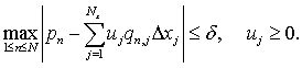 (11)
(11)
In (11):;
.
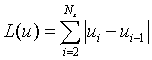
Experimental setup for image formation f(s)
A sketch of the setup is presented in Fig. 2. All components installed at the top row are part of the spectrometer of millimeter/submillimeter range of the Institute of General Physics named after A. M. Prokhorov of RAS[8]. The coordinate tables are produced by the Company "SPF Electric Drive"[9]. The coordinate tables drivers movement and the data acquisition are realizing by means of the universal software complex developed in IRE RAS[10].
The selected scheme of the movement of the telescope imitator in relation to fixed BWT and the movement of the Golay cell in relation to the telescope imitator in each position of the telescope imitator in the horizontal plane along lines perpendicular to the axis quasi-optical tract, during the measurements process, is presented in Fig.3.
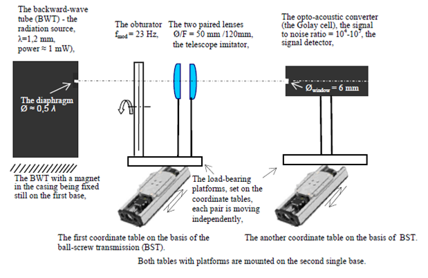
Fig.2. The sketch of experimental setup for the image formation modeling.
It is clear that the described experimental setup does not give direct opportunities to obtain the core ![]() of the equation because it uses one source and one detector. To simulate the set of sources it has proposed a mechanism to move the "telescope imitator", and to simulate a set of detector it has proposed a mechanism to move the detector. This method has several advantages over the actual use of multiple sources and multiple detectors. It is obvious, first, that this method can achieve the identity of radiation sources and detectors of the measuring system. Secondly, such a scheme of the experiment, of course, reduces the cost of the required equipment.
of the equation because it uses one source and one detector. To simulate the set of sources it has proposed a mechanism to move the "telescope imitator", and to simulate a set of detector it has proposed a mechanism to move the detector. This method has several advantages over the actual use of multiple sources and multiple detectors. It is obvious, first, that this method can achieve the identity of radiation sources and detectors of the measuring system. Secondly, such a scheme of the experiment, of course, reduces the cost of the required equipment.
Using the described setup, there were performed a series of experiments, the results of which made it possible to construct the response function of the recording apparatus (the core of the equation ![]() ). The function
). The function ![]() is shown in Fig. 4.
is shown in Fig. 4.
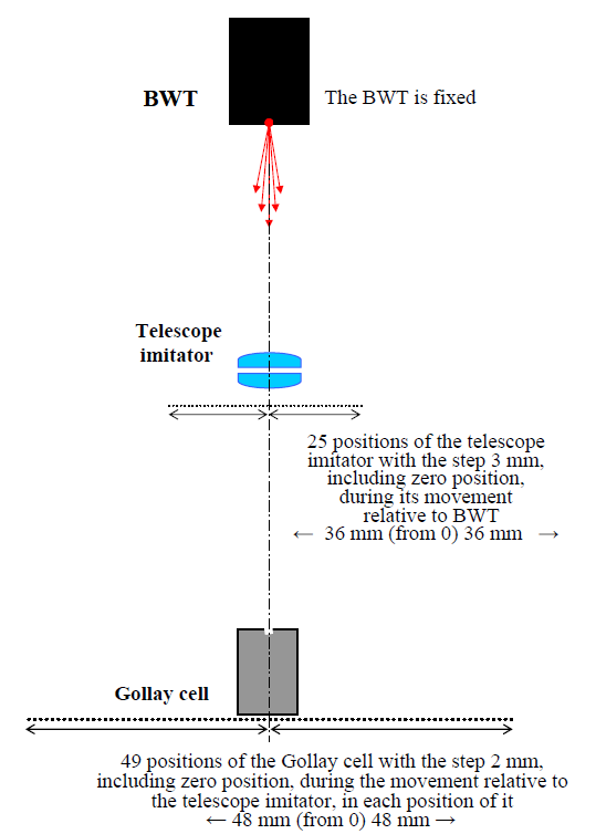
Fig. 3. The scheme of reciprocal movements of parts of the experimental setup (in a plan view).
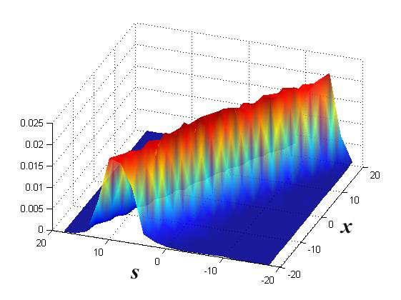
Fig. 4. The graph of the function ![]()
The simulation results
To demonstrate the capabilities of the developed method of reconstruction of the field of sources (radiation sources density) there had been done a series of model calculations within the model of described above for one-dimensional experiment.
As hardware function there was used the built kernel ![]() of the integral equation (4) shown in Fig. 4. The field sources were asked in the form of two point sources located at different distances from each other within the diffraction blur of the recorded image.
of the integral equation (4) shown in Fig. 4. The field sources were asked in the form of two point sources located at different distances from each other within the diffraction blur of the recorded image.
It is shown in Fig. 5 an example of calculation, when the distance between sources is 1 mm, and the noise level is 2%. To the Fig. 5,a - the image recorded by the line of detectors, to the Fig.5,b the result of the reconstruction of the field of sources. The abscissa in these figures is the distance in mm. On the Fig. 5,a is the position of detectors (line ![]() in Fig.1), on the Fig.5,b is the position of sources (line
in Fig.1), on the Fig.5,b is the position of sources (line ![]() in Fig. 1).
in Fig. 1).
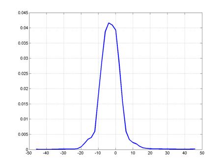
Fig.5,a. The image obtained using the line of detectors.
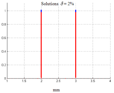
Fig.5,b. Exact (blue) and reconstructed field of sources (red).
It is shown in Fig. 6 an example of calculation, when the distance between the sources is equal to 0.1mm, and the noise level is 2%. To the Fig. 6,a – the image recorded by the line of detectors, to the Fig. 6,b the result of the reconstruction of the field sources. The abscissa in these figures is the distance in mm.
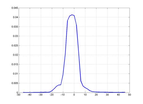
Fig. 6,a. The image obtained using the line of detectors
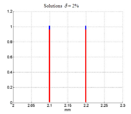
Fig. 6,b. Exact (blue) and reconstructed field of sources (red).
Note, that the half-width of the diffraction blur in the above examples is of the order of 15mm. Thus, in the first example, the resolution of the two sources exceeds the blurred image by 15 times, and in the second one – by 150 times. For the selected noise level (2%) resolution 0.1 mm is a limit. With the increase of noise level up to 5-7% limiting resolution deteriorates approximately linearly.
Conclusion
It is important to note that the results obtained are first, the provisional nature and require further investigations, both in experimental plan and in terms of reconstruction algorithms of the field of sources. It is also important to say, that the transition to real two-dimensional images requires the use of more complex algorithms and significantly more powerful (including hybrid) computing hardware, in particular, due to the fact that hardware features in the two-dimensional case are a function of four variables and its determination requires a huge amount of calculations.
References
1. A.N. Vystavkin, S.E. Bankov, M.E. Zhukovskiy, S.V. Podoljako, The patent of RF №2533502, “The method of the image formation with the subdiffraction resolution”, priority date 20.02.2013.
2. A.N. Tikhonov, V.Ja. Arsenin,“Methods of solution of ill-posed problems”, Moscow, “Nauka”, 1986.
3. V.P. Zagonov, S.V. Podoljako, “Some algorithms of approximate solution of integral equations of the first kind in the presence of a priori restrictions”, Mathematical Modeling”, 1992, v. 4, №4, p. 89-100.
5. V.P. Zagonov, “On approximation of nonsmooth solutions to ill-posed problems in the Hausdorff metric”, Preprint of IAM named after M.V. Keldysh, 1990, №158.
6. Ju.A. Kriksin, “Numerical solution of integral equations of the first kind by the method of local residual”, Preprint of IAM named after M.V. Keldysh, 1986, № 52.
7. M.E. Zhukovskiy, G.-R. Jaenisch, A. Deresch, S.V. Podoliako, Mathematical modeling of radiography experiments. Beitrag zu einem Tagungsband: 18th WCNDT - World conference on nondestructive testing (Proceedings) (2012), Paper 305, 1-7 ISBN 978-0-620-52872-6.
8. N.A. Irisova, The metric of submillimeter waves, Vestnik of Soviet Academy of Sciences, 1968, issue 10, p. 63.
9. SPF Electric Drive, http://www.eprivod.ru/index.htm.
10. I.A. Cohn, A.G. Kovalenko and A.N. Vystavkin, Experimental research control software system, Journal of Physics: Conference Series, vol. 510, no. 1, p. 012004. IOP Publishing, 2014.
References 1- 6, 8, 9 are in Russian.