| "JOURNAL OF RADIO ELECTRONICS" N 2, 2000 |
ASYMPTOTIC METHOD FOR PREDICTING ERROR PERFORMANCE PARAMETERS AND OBJECTIVES FOR CONSTANT BIT RATE DIGITAL PATHS CARRIED BY DIGITAL RADIO-RELAY SYSTEMS
Vladimir Minkin, Alexander Voschinin
Radio Research & Telecommunication Institute (NIIR)
Received February 22, 2000
At present there are two concepts to evaluate the error performance parameters and objectives for digital radio-relay systems forming a part of SDH-network. The parameters and objectives for systems below the primary rate are defined in ITU-T Recommendation G.821 [1] while those for systems at or above the primary rate are specified in ITU-T Recommendation G.826 [2]. For the time being the design of radio-relay links at or above the primary rate was based on ITU-T Recommendation G.821 approach. For both design and maintenance of the digital links it is important to determine converting statistics and establish relations between error performance objectives according ITU-T Recommendations G.821 and G.826. In the present paper this problem is solved with asymptotic approach based on normal approximation to the binomial distribution. Under this, for time-invariant number of errors per burst and bit error ratio, BER(t), distribution, multipliers for converting parameters in accordance with Recommendation G.821 into parameters in accordance with Recommendation G.826 are found. For the complex case of time-variant characteristics the asymptotic method for predicting error performance parameters is developed. Proposed evaluating algorithm is numerically verified with estimation of block error performance parameters on a design of radio-relay hop. The BER(t) distribution mask that could allow meeting error performance objectives for a hop has been defined using different propagation and equipment parameters.
Error performance objectives for a constant bit rate digital path at or above the primary rate carried by digital radio-relay systems which may form part of the international and national portions of a 27 500 km hypothetical reference path are defined by ITU-R Recommendations F.1092 [3] and F.1189 [4] based on ITU-T Recommendations G.826.
To simplify in-service measurements the Recommendation G.826 is based upon a block-based measurement concept using error detection codes inherent to the path under test and considers the following block-based events:
Error performance parameters related with above events are defined as:
A path fails to satisfy this Recommendation if any parameter exceeds the allocated objective in either direction at the end of the given evaluation period. The suggested evaluation period is 1 month.
At the same time the radio-relay equipment specifications define receiver level threshold based on Bit Error Ratio (BER) criterion (BER=10-3). This approach was widely used for a path design in ITU-R Recommendation P.530-7 [6] because old ITU-R Recommendation F.594 [7], F.634 [8], F.696 [9] and F.697 [10] were based on ITU-T Recommendation G.821 where BER criteria were used for error event definitions and SES event was declared at BER=10-3. Also for the time being there have been published only a few experimental measurement results based upon errored blocks and there are a lot of publications containing experimental results related with BER. As it is mentioned in the ITU-R Recommendation P.530-7 if requirements in Recommendation G.826 have to be met there is a need for prediction methods that are based on estimating block errors rather than bit errors could allow to calculate the ESR, BBER and SESR objectives.
For this it is important to have a method and procedure to convert BER statistics into block-based event statistics. A number of such methods have been recently proposed [11], [12] and [13]. Basing on different sets of assumptions and input data above methods provide numerical evaluation of error performance parameters. Being tested with real data these methods proved to be quit convenient. However, to investigate the basic properties of different error performance parameters it is important to establish analytical relations between different criteria.
In this paper based on a normal approximation to the binomial distribution the asymptotic approach to this problem is developed. The received equations give simple relationships between block based error performance parameters and could be useful for the amendment of ITU-R Recommendation P.530. The BER (t) distribution mask has been developed to estimate possibility for a hop with known propagation and equipment parameters to meet the error performance objectives.
The paper is organized as follows. In section 2 asymptotic formulas for probability of block-based events as a function of BER are derived. Time dependence of BER and probability of basic events is investigated in section 3. Asymptotic formulas for ESR, SESR and BBER are obtained in section 4. Under assumption that mean error burst length and BER distribution are time invariant a simple converting multipliers are derived in section 5. For more complicated case of time variant characteristics the prediction method for error performance parameters is developed in section 6 where the BER(t) distribution mask has been defined. Concluding remarks are presented in section 7.
2. ASYMPTOTIC PROBABILITY OF BASIC EVENTS
Relationship between error performance parameters and BER can be evaluated employing either Poisson distribution or Neyman-A contagious distributions of bit errors within a burst. It is shown in [11] that either approach leads practically to identical results. Since Poisson distribution is more pragmatic and provides useful results with minimal complexity henceforth Poisson distribution is applied.
2.1. Probability of an errored block PEB
Assuming a Poisson distribution of errored bursts probability of an errored block PEB can be expressed in the form
|
PEB=1-exp(-NB BER/a )=1-exp(-BER/t ), |
where BER is a bit error ratio, NB is a number of bits per block, a is an average number of errors per burst (a ³ 1), constant t = a /NB is used to evaluate a change rate of the exponent. Basing on the fact that exponent runs from 0 up to 0.95 when its argument changes from 0 up to 3t we can state that
This statement, which explicitly connects working range of PEB with block size and number of errors per burst is useful when numerical integration should be performed.
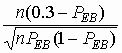
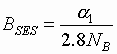
Due to above given definition of SES this event occurs when number of errored blocks per second is greater than 30%, i.e. when PEB³ 0.3. It allows to write an expression for equivalent BER threshold BSES for SES to occur as
To compare different distribution models numerical values of BER threshold normalized to the mean burst a =1 are given in Table 1 for different block sizes under Poisson, binomial and uniformed distribution.
Table 1. Threshold BER for a SES to occur for different block size and distribution models
|
Distribution models |
NB=18 792 bit |
NB=6120 bit |
NB=2048 bit |
|
Poisson |
1.83 10-5 |
5.50 10-5 |
1.74 10-4 |
|
Binomial |
1.88 10-5 |
5.64 10-5 |
1.78 10-4 |
|
Uniform |
1.54 10-5 |
4.63 10-5 |
1.46 10-4 |
From the Table 1 it can be seen that the difference between BER threshold values under Poisson and binomial distribution is insignificant. As to the uniform distribution it yields more stringent requirements for system. However, the data in the Table 1 shows relatively low sensitiveness of threshold to the type of distribution.
2.2. Probability of an errored second PES
With probability of errored blocks given by equation (1) it is possible to define a probability PES of an errored second as
where n is a number of blocks per second. Under this, based on the �3t rule� we can conclude that
i.e. the probability of an errored second PES runs interval 0£ PES£ 0.95 where probability of errored blocks PEB has order 1/n. Under this a linear approximation to equation (1) is valid and hence we can write expression
which is practically accurate (error of approximation is less than 1/n2). Comparing expression (1) and (5) we can conclude that for any fixed value of BER and other things equal the following relation is valid
With equation (6) it is easy to set the correspondence between different values of BER which yields the same probability of errored blocks and errored second PEB=PES. For example, for path VC-4 with NB=18720, n=8000 assigning PEB=PES=0.3 from Table 1 for Poisson distribution we have PEB(BER=1.83 10-5)=0.3. Dividing argument by n=8000 in accordance with equation (6) we get
2.3 Probability of severely errored seconds PSES
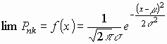
To evaluate probability of errored seconds it is necessary first to define the probability Pnk of k errored blocks in total of n blocks. It can be found by use of binomial distribution as
It is known [14] that normal distribution with mean m and variance s2 defined as
provides a very accurate approximation to the binomial distribution (8) when n is large. It allows to write the limiting form of equation (8) when n tends to infinity as
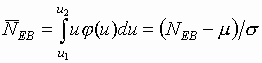
Here random normal variable x in expression (11) has a sense of number of errored blocks per second. Considering all cases when ratio k/n is greater than or equal to 0.3 the probability PSES can be calculated as a sum
which with equation (10) can be replaced by integral, i.e. expression for PSES can be written as
As before, f(x) is the probability density function of normal random variable x with mean m and variance s 2.
The properties of integral (12) have been investigated in details in Appendix A. Main conclusions can be summarized in the set of following statements:
where F(u) is cumulative standard normal distribution of random variable u with zero mean and variance equal to 1, u1 is normalized lower limit of integral (12).
Expressions (13) and (14) reveal that PSES curve that is exponential in shape changes from 0 to 1 in very narrow BER interval. For example, for VC-4 path with NB=18720 bits, n=8000 blocks/s, PSES changes from 0.005 to 0.995 when BER=1.83 10-5± 7.7 10-7. For path with NB=2048 bits and n=1000 blocks/s respective interval is defined as BER=1.74 10-4± 2.1 10-5
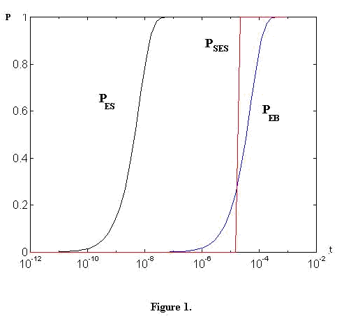
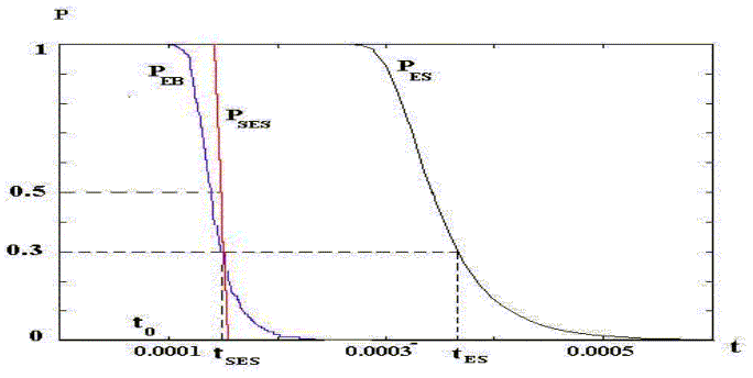
Thus, expression (14) analytically verifies usually accepted assumption that function PSES is nearly step function. The PEB, PES and PSES curves vs. BER are shown for VC-4 path in the Figure 1.
3. BER AND PROBABILITY OF BASIC EVENTS AS FUNCTIONS OF TIME
3.1. Cumulative BER distribution
In real radio-relay links BER depends on propagation conditions and can be represented by a stochastic process. Cumulative distribution t (BER) of this process evaluates worst month time (taken as relative time t, which is equal to 1 for the whole observation interval) when BER exceeds the given BER value.
A precise relationship between time t and BER can be obtained only from direct measurements on considered radio link. Another way is to derive the distribution t (BER) from distribution t (V) of fade margin V that could be known or proposed for given path.
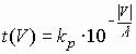
It is shown in [15] that for low fraction of the distribution of fade margin V
(for ½V½> 25 dB) can be described as
where t is relative worst month time when input fade margin V
exceeds the given value,
kp- coefficient adjusted to considered path,
l - coefficient which depends on frequency range and diversity mode.
From real link measurements it could be consider that, for
example,
l = 5 for multipath fading and space
diversity,
l = 10 for multipath fading and
single reception as well as for fading due to rain at some paths in frequency
ranges about 11 GHz,
l = 20-25 for fading due to rain at
some paths in frequency range 18 GHz and higher.
Let also assume that the relationship between BER and fade margin V[dB] could be approximated by equation
where j is a constant adjusted to the link, coefficient b reflects the rate of change of the function BER(V).
In Figure 2 some typical curves described by equitation (16) are presented. For a generality on an abscissa axis we shall consider relative meanings ½V- V0½ , where V0 - fade margin,dB, appropriate to a receiver input level at B0=10-3.
Figure 2.
For all curves j = -3 and the curve slope b is defined as
a) 
b)
c)  only fir systems with FEC with a large code gain.
For prediction of error performance parameters it is necessary to derive distribution t(BER) from expressions (15) and (16). To solve this problem let�s suppose that there is given a reference point (t0, V0, B0) on the distribution curves (15) and (16). Under this assumption after several manipulations it is possible to avoid unknown coefficients k and j from expressions (15) and (16) and to combine them into the unique distribution t(BER).
Indeed, substituting the pair of coordinates (t0, V0) into equation (15) we can write for unknown coefficient k
![]()
With this expression we can represent distribution (15) in the form
which does not include coefficient k.
Using the pair (V0, B0) after similar manipulation equation (16) can be written as
Comparing equation (17) and (18) we can see that both of them include the term {| V0| -| V| }. Its explicit expression can be easily found from equation (18). Substituting it into (17) and taking inverse function we can write resulting distribution BER(t) as
where the index m=b l is supposed to be a known positive number greater than one.
As it follows from the above given expression the BER value falls m decades when relative time changes for one decade, i.e. in loglog scale relation (19) is represented by a straight line with the slope m.
As a rule distribution (19) could not be valid for whole range of relative time [t0, 1]. For this reason to describe actual relation BER(t) more precise, the whole range of relative time [t0, 1] can be divided into several line segments with different corresponded slope m. Resulting relation BER(t) in this case is represented by piece- wise function (Application of 3-points distribution will be given in section 6).
3.2 Probability of basic events as a function of time
If relation BER (t) is known, the probability of block events can be represented as a function of time percentage t. For example, if BER distribution BER (t) is given by equation (19) then by substitution in it BER in expressions (1), (3) and (13) we get respective probability as a function of time.
|
PEB(t)=1-exp[-NB (B0/a )(t0/t)m] |
|
|
PES(t)=1-exp[-n NB (B0/a )(t0/t)m] |
|
|
PSES(t)=1-F[u1(t)], |
where u1(t) = 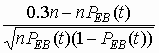
In Fig. 3 the curves PEB(t), PES(t) and PSES(t) are shown for VC-4 path with B0=10-3, t0=0.0001, a =1 and m=10.
Figure 3
Three specific points are shown in Fig.3, namely point t0, corresponded to the maximum BER value equal to B0=10-3, point tSES corresponded to the threshold BSES where PEB=0.3 and point tES where PES=0.3.
4. DETERMINATION OF ERROR PERFORMANCE PARAMETERS
Under explicitly given time dependent probabilities PEB(t), PES(t) and PSES(t) evaluation of error performance parameters can be done by using integration of respective functions over relative time interval [t0, 1]. Indeed, for ESR and SESR parameters we can write
where the lower limits of integrals t0 is the fraction of time when BER exceeds its highest value equal to B0=10-3, and the upper limit, which is equal to one, corresponds to the total relative observation time (any month).
Recommendation ITU-T G.826 define BBER as the ratio of errored blocks to total blocks during available seconds, excluding all blocks during SES. In Appendix B with asymptotic approach it is shown that BBER can be evaluated as integral
where the lower integration limit is taken as time percentage t1 corresponded to the SES threshold BSES where PEB=0.3. For t>tSES there are no SES. The multiplier 1/(1-SESR) in expression (25) reflects the fact that all blocks during SES are excluded from consideration. Equation (25) is useful for two reasons. First, it yields the implicit, easily interpreted relationship between BBER and probability of errored blocks PEB and the second, it essentially simplifies numerical integration.
Geometrically, integrals (23), (24) and (25) correspond to the area bounded by the respective curves PES(t), PSES(t) and PEB(t) shown in Fig. 3.
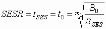
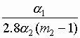
Taking into account that PSES is nearly step function a simple relation can be applied to evaluate SESR, namely
which is valid with high accuracy. SESR value due to equation (26) equal to area of rectangle with base tSES and height equal to one. It can be seen from Fig. 2 that it is very close to the area bounded by curve PSES(t), i.e. to the exact SESR value. The value of tSES related with SES threshold can be found for given m with equation (19) by substitution BER=BSES as
Concerning BBER parameter it can be observed that for PEB<0.3 linear approximation to probability PEB given by expression (1) is valid , i.e. we can write
Assuming distribution BER(t) in the form of (19) and using approximated relation (28) integral (25) can be evaluated analytically as
Final form of equation (29) is obtained with equation (2) taking into account that the value of integral under its upper limit is negligible small in comparison with its value under the lower limit. (That is correct if tSES and the impact from BER �tail� (when, e.g., BER < 10-12) are negligible small and m and a are constant over the interval [tSES , 1]).
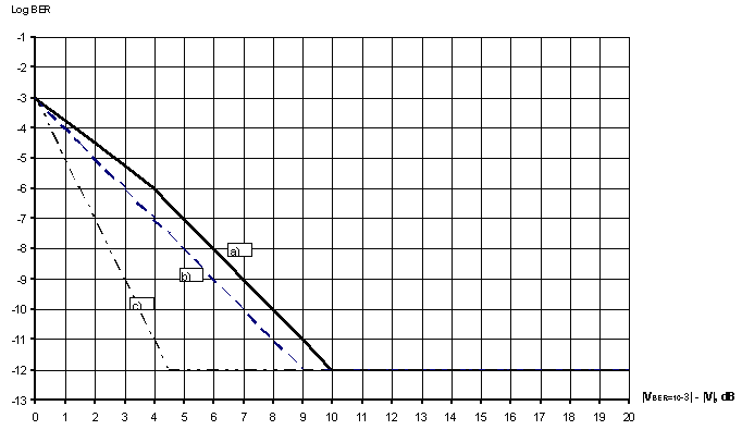
In Fig. 4 the exact curve PEB(t) and its linear approximation (28) are shown for the same data as for Fig. 3.
The shadowed area in Fig. 4 corresponds to the exact value of BBER. Linear approximation of PEB(t) represented by upper curve adds the narrow band to this area. Resulting overestimation of BBER for either path type does not exceed 7%.
It should be mentioned that using distribution BER(t) in the form of (19) we practically have considered only part of the BER(t) distribution without BER �tail�.
4. DETERMINATION OF ERROR PERFORMANCE PARAMETERS
Under explicitly given time dependent probabilities PEB(t), PES(t) and PSES(t) evaluation of error performance parameters can be done by using integration of respective functions over relative time interval [t0, 1]. Indeed, for ESR and SESR parameters we can write
where the lower limits of integrals t0 is the fraction of time when BER exceeds its highest value equal to B0=10-3, and the upper limit, which is equal to one, corresponds to the total relative observation time (any month).
Recommendation ITU-T G.826 define BBER as the ratio of errored blocks to total blocks during available seconds, excluding all blocks during SES. In Appendix B with asymptotic approach it is shown that BBER can be evaluated as integral
where the lower integration limit is taken as time percentage t1 corresponded to the SES threshold BSES where PEB=0.3. For t>tSES there are no SES. The multiplier 1/(1-SESR) in expression (25) reflects the fact that all blocks during SES are excluded from consideration. Equation (25) is useful for two reasons. First, it yields the implicit, easily interpreted relationship between BBER and probability of errored blocks PEB and the second, it essentially simplifies numerical integration.
Geometrically, integrals (23), (24) and (25) correspond to the area bounded by the respective curves PES(t), PSES(t) and PEB(t) shown in Fig. 3.
Taking into account that PSES is nearly step function a simple relation can be applied to evaluate SESR, namely
which is valid with high accuracy. SESR value due to equation (26) equal to area of rectangle with base tSES and height equal to one. It can be seen from Fig. 2 that it is very close to the area bounded by curve PSES(t), i.e. to the exact SESR value. The value of tSES related with SES threshold can be found for given m with equation (19) by substitution BER=BSES as
Concerning BBER parameter it can be observed that for PEB<0.3 linear approximation to probability PEB given by expression (1) is valid , i.e. we can write
Assuming distribution BER(t) in the form of (19) and using approximated relation (28) integral (25) can be evaluated analytically as
Final form of equation (29) is obtained with equation (2) taking into account that the value of integral under its upper limit is negligible small in comparison with its value under the lower limit. (That is correct if tSES and the impact from BER �tail� (when, e.g., BER < 10-12) are negligible small and m and a are constant over the interval [tSES , 1]).
In Fig. 4 the exact curve PEB(t) and its linear approximation (28) are shown for the same data as for Fig. 3.
The shadowed area in Fig. 4 corresponds to the exact value of BBER. Linear approximation of PEB(t) represented by upper curve adds the narrow band to this area. Resulting overestimation of BBER for either path type does not exceed 7%.
It should be mentioned that using distribution BER(t) in the form of (19) we practically have considered only part of the BER(t) distribution without BER �tail�.
5. SIMPLE CONVERTING METHOD FOR CONSTANT m and a
Above given asymptotic expressions (23), (26) and (29) provide theoretical base to develop asymptotic prediction method of error performance parameters due to ITU-T Recommendation G.826 [1]. To improve the accuracy of method any available information related with given link should be included into consideration. For example, as much as possible precise presentation of BER(t) in the form of piece wise function is of great importance. It is also necessary to take into account time dependence of average number of errors per burst a . Due to the simple structure of integrals (23), (24) and (26) this information can be involved in calculation without any difficulties.
The problem of converting of bit error-based measurements into ESR, SESR and BBER parameters can be reduced to the determination of converting multipliers k, k1(kES) and k2(kBBE) such that
Let�s find k, k1, k2, kES and kBBE under the following assumptions:
Note: It should be mentioned again that for ESR and BBER relationships (30) are valid under an assumption that the impact of BER �tail� is negligible small.
Below in this section simple converting method based on multipliers k, k1 and k2 is considered.
5.1 SESR evaluation.
Using expression (26) for SESR and expression (2) and (27) for t1 we can readily get the converting relation
with converting multiplier k defined asThe values of k calculated for selected block size NB,
index m and mean burst a are presented in the
Table 2
(B0= 10-3).
Table 2. Converting multiplier �k� for SESR
|
NB=18 792 bit |
NB=6120 bit |
NB=2048 bit |
|||||||
|
m |
5 |
10 |
20 |
5 |
10 |
20 |
5 |
10 |
20 |
|
a = 1 |
2.2 |
1.5 |
1.2 |
1.8 |
1.3 |
1.15 |
1.4 |
1.2 |
1.09 |
|
a = 2 |
1.9 |
1.4 |
1.18 |
1.5 |
1.24 |
1.1 |
1.1 |
1.1 |
1.05 |
|
a = 5 |
1.6 |
1.3 |
1.12 |
1.3 |
1.13 |
1.0 |
1.0 |
1.0 |
1.0 |
|
a = 10 |
1.4 |
1.2 |
1.09 |
1.1 |
1.05 |
1.0 |
0.9 |
0.9 |
0.97 |
The SESR estimation given by equation (31) is nearly exact and for this it can be applied even for an accurate evaluation of SESR parameter.
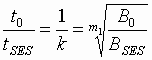
The equations (31) and (32) allow to solve the reverse problem - to estimate what should be the t0 value if a path meets the SESR0 value that denotes the required one for SESR objective
t0 ³ SESR0
/k = SESR0  =
SESR0
=
SESR0  .
.
The t0 value may be used for path design purposes using the known received threshold at B0= 10-3 for Vmin calculations in ITU-R Recommendations P.530[2] and F.1093[3].
5.2 ESR evaluation.
The exact value of ESR parameter can be found with equation (23) which even under above assumptions is not linear with respect to time t0. For this reason to find multiplier k1 the following rough estimation of integral (23) is applied
where tES is time percentage when probability of error seconds PES(t) exceeds the value 0.3. Replacement of integral (23) by the equation (33) is equivalent to the approximation of exponent PES(t) in figure 3 by the step function with the jump at the point tES. Under this, instead of area bounded by the curve PES(t) that is exact value of ESR, we have an area of rectangle with the base tES. This yields to slight overestimation of ESR value.
To calculate the value tES the relationship (6) can be applied. From equation (6) it follows that PES=0.3 if BER value is equal to B2=BSES/n. Substituting it in distribution (19) we have
Simple relation between tES and tSES together with equation (31) yields the following converting formula for ESR
where k is given by expression (31). The values of multiplier kES for selected combinations of n and m are presented in the Table 3.
Table 3. Converting multiplier kES for ESR
|
n (blocks/s) |
1000 |
8000 |
|
m= 5 |
4 |
6 |
|
m=10 |
2 |
2.5 |
|
m=20 |
1.4 |
1.6 |
The k1 values can be easily found by multiplying columns of Table 2 by appropriate factor kES from Table 3 or directly from expression (32) and (35). Though ESR estimation due to (33) have been referred as a rough one, practically in worst-case error does not exceed 20%.
If we have defined the m and a values correctly the receiving result should be less than measured ESR value and the difference between estimated and measured ESR values could be used for real residual BER �tail� (RBER) impact estimation.
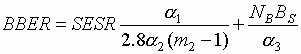
5.3 BBER evaluation.
For determination of multipliers k2 and kBBE in expression (30) the approximation (29) for BBER can be used. Under this, using expression (2) for BSES and (31) for tSES we can represent BBER as
where multiplier kBBE is defined as
The values of kBBE are given in the Table 4.
Table 4. Converting multiplier kBBE for BBER
|
m |
5 |
10 |
20 |
|
kBBE |
0.09 |
0.04 |
0.019 |
The k2 values can be easily found by multiplying columns of Table 2 by appropriate factor kBBE from Table 4. As it was mentioned before, the evaluation of BBER with use of converting formula (36) for worst case does not exceed 7% (without taking into account the RBER �tail� impact).
5.4 Relations between error performance parameters.
Simple manipulations with equations (31), (35) and (37) reveal the following relations:
which are invariant to the time percentage t0, block size NB and average number of errors per burst a .
For example, the ESR/SESR and BBER/SESR relations between error performance parameters under index m=5 and m=10 are calculated below:
Table 5. Relationship between error performance parameters
|
m |
5 |
10 |
||
|
n |
1000 |
8000 |
1000 |
8000 |
|
ESR/ SESR |
4 |
6 |
20 |
2.5 |
|
BBER/ SESR |
0.09 |
0.09 |
0.04 |
0.04 |
|
ESR/ BBER |
44 |
67 |
50 |
62 |
Let�s compare equations (38) and (39) using the relationship between objectives SESR0 , ESR0 and BBER0 taken from Table 1/ G.826 in the ITU-T Recommendation G.826.
Table 6. Relations between error performance parameters according ITU-T Recommendation G.826
|
Rate (kbit/s) |
2048 |
48 960 |
150 336 |
|
Block size |
2048 bits |
6 120 bits |
18 792 bits |
|
Blocks/second |
1 000 |
8 000 |
8 000 |
|
ESR0/ SESR0 |
20 |
37.5 |
80 |
|
BBER0/ SESR0 |
0.1 |
0.1 |
0.1 |
It could be seen from Table 6 that the most critical is the relationship BBER/ SESR.
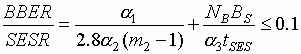
Suppose that BER(t) distribution is described by expression (19) with a constant index m and a path meets SESR objective. Under this assumption using the relation (39) and BBER0/ SESR0 ratio from Table 6, we can state that the path will meet the BBER0 objective if the following inequalities are satisfied.
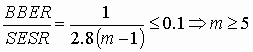
Experimental date shows that the index could vary in the range m = 5�20. It means that the relationship BBER/ SESR could not be less than 0.019 for radio-relay systems without space diversity and not less than 0.04 for radio-relay systems with space diversity (the BER �tail� impact is here ignored).
6. PREDICTION METHOD FOR TIME-VARIANT m and a
The simple converting method developed in section 5 is based on assumptions that index m and mean burst a are constant. However, in real radio-relay links both index m of BER distribution and average number of errors per burst a are time variant. Under this it should be developed the prediction method with greater level of complexity to take into consideration detail information related with mean burst a and distribution BER(t). It is also important to evaluate the contribution of the �tail� of BER(t) distribution in error performance parameters. Usually, a �tail� is referred to that part of BER(t) where BER(t) is constant. Usually mainly an equipment residual BER and some type of interference but also a number of unpredictable reasons define this part.
To take into consideration all these effects to estimate errors performance parameters of given path with known block size NB and number of blocks per second n the following assumptions are made
t0 is
percentage-of time corresponded to the highest BER value B0 ,
tSES corresponds to the SES threshold BSES
and
tS is a
�tail� starting point related with BS=10-10�10-13
.
,
(41)
under tSES£ t£ tS
,
under tS£ t
6.1 Evaluating algorithm.
Let�s evaluate error performance objectives for an one hop path under given relation (41), known indexes m1, m2, m3 and average number of error per burst a 1, a 2, a 3 . It is also necessary to define the coordinates of characteristic point. It is mentioned in the current ITU-R Recommendation P.530 that the prediction methods are all based on a definition of outage as BER above a given value, i.e., 10-3, for meeting requirements set out in Recommendation G.821[4]. If requirements in Recommendation G.826 have to be met there is a need for prediction methods that are based on estimating block errors rather than bit errors. In order to meet the requirements in G.826 the link should be designed to meet another BER than 10-3.
It means that using the above mentioned prediction methods we could receive for the path under consideration for B0 =10-3 only the coordinate of characteristic point t0 and the coordinates of another characteristic point [BSES, tSES] should be calculated.
In this case the following step-by-step evaluating procedure is given.
If it is possible using the prediction methods to calculate tSES based on the BSES threshold known from DRRS equipment specification we could take them as co-ordinates of the characteristic point [BSES, tSES].
In both cases we could continue the further consideration from the point with coordinates [BSES; tSES] where tSES = SESR.
Approximate value of ESR can be found in accordance with (35) as
The value BS can be considered as 10-10¸ 10-13. Geometrically contribution of the tail is equal to the area of rectangle with base (1-tS) and the height equal to the appropriated probability at the point tS. Under this, the contributions of the tail to the error performance parameters following equations are applied
The contribution to SESR is equal to zero because PSES is nearly step function.
Then using approximate relation (44) and relations (45), (46) and (47) we could estimate ESR and BBER taking into account the �tail� effect and considering ts<<1
6.2 Design of radio-relay link
Above procedure can be basically applied also for the design of radio-relay
links. It is assumed that BER (t) distribution is a 3-point piece-wise function
with each part of the distribution described by equation (41).
Then suppose that a path has been designed to meet SESR (=tSES)
objective according ITU-T Recommendation G.826 or respective ITU-R
Recommendations.
It is necessary to determine a bit-error probability mask BER (t), defined by
values of mi and a i in
the distribution (41), in a such way that digital
transmission would meet the above mention objectives taking into account the
relationship from Table 6.
Step-by-step procedure
Calculations are accomplished from small values of percentage-of-time to the higher one when the BER �tail� effect is neglected during the first steps.
Values for BSES /a 1 and k could be taken from Tables 1 and 2 respectively.
For of m2 ![]() we have
we have ![]() <
<
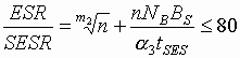
![]() 6.
Under this the ratio ESR/SESR £ 80 for VC-4, £
37,5 for VC-3 and £ 20 for 2048 kbit/s are met
when
6.
Under this the ratio ESR/SESR £ 80 for VC-4, £
37,5 for VC-3 and £ 20 for 2048 kbit/s are met
when
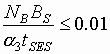
First of all let�s estimate under what value BS / a 3 we could consider the second part of the sum negligible for NB = 18792 , 6120 or 2048.
Then taking it into account we could receive that
![]() ,
if
,
if 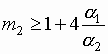 ,
,
for a 1= a 2
![]()
a 1=2a 2
![]()
Comparing inequalities (50) and (52) one could see that for paths VC-4/VC-3 and 2048 kbit/s ITU-T Recommendation G.826 objectives could be met if
Let consider BER(t) mask for a VC-4 path under different a and m.
In the Table 7 relative values of t0/tSES and ts/tSES are given for
m=5, 10 and 20 under
1) a 1=a 2=a 3=1 (B0=10-3; BSES=2x10⁻⁵;)
2) a 1=a 2=10, a 3=1 (B0=10-3; BSES=2x10⁻⁴; Bs=10-12).
The Bs=10-12 value is taken as the threshold value that could allow to meet (53) even for a 50 km hop from 50-hops 2500 km international VC4 path, block size NB=18792 bits, number of blocks n=8000 blocks/s.
Error performance objectives for given path is defined as SESR0=2.4 10-6, ESR0=1.9 10-4, BBER0=2.4 10-7.
For other paths this value could be more than 10-12.
Relative values t0/tSES and ts/tSES for a 50 km hop from 50-hops 2500 km international VC4 path for variants 1) and 2) could be found in Table 7.
Table 7. Relative values t0/tSES and ts/tSES
|
t0/tSES |
ts/tSES |
|||||
|
m |
5 |
10 |
20 |
5 |
10 |
20 |
|
for 1) |
0.46 |
0.68 |
0.82 |
30 |
5.5 |
2.3 |
|
for 2) |
0.72 |
0.85 |
0.92 |
47 |
6.8 |
2.6 |
The BER (t) mask based on Table 7 is given in Fig. 5.
Considering the Figure 5 it could be seen that the average number errors per burst a i has less impact on the mask than the slope mi especially with mi increasing.
As an example the dotted line in the Figure 5 shows the BER(t) mask for following parameter:
m1 = 7.5; a 1=10 t Ì [t0,tSES]
m2 = 10; a 2= vary from 10 to 2 t Ì [tSES,tS] (56)
a 3=2 t ³ tS
The above-considered results have shown that it will be useful to include in DRRS technical specification the following additional parameters:
7. CONCLUSIONS.
We have presented the asymptotic method for predicting error performance parameters of terrestrial digital radio-relay links based on normal approximation to the binomial distribution. With analytical expressions obtained for probability of basic events it has been proved that probability PSES is equal to 0.5 under 30% PEB threshold. The simple relation between 30% thresholds PEB and PES has been established. It was shown that SES(BER) is practically a step function and strongly depends on average error burst value for BER=10-3 �10-6 and a block size.
The simple converting method has been developed for time variant case with constant index of distribution BER (t) and invariant mean burst length. Under this, analytical relations depending on number of blocks per second and index of BER distribution between ESR, SESR and BBER have been found.
The prediction method and evaluating step-by-step procedure have been developed for piece wise distribution BER (t) with time variant average number of errors per burst has been also elaborated.
The numerical relationship between propagation and equipment parameters that could allowed to meet error performance objectives for 2048 kbit/s, VC-3 and VC-4 paths according ITU Recommendations have been also presented as well as the relative BER(t) mask.
It was shown that if the residual BER < 10-12:
References
|
ITU-T Recommendation G.826 |
Error performance parameters and objectives for international bit rate digital paths at or above the primary rate. ITU. Geneva. 1999. |
|
|
ITU-T Recommendation G.821 |
Error performance of an international connection forming part of an integrated services digital network ITU. Geneva. 1996. |
|
|
ITU-R Recommendation F.1092 |
Error performance objectives for constant bit rate digital paths at or above the primary rate carried by digital radio-relay systems, which may form part of the international portion of a 27500 km hypothetical reference path. ITU. Geneva. 1997. |
|
|
ITU-R Recommendation F.1189 |
Error performance objectives for constant bit rate digital paths at or above the primary rate carried by digital radio-relay systems which may form part of the national portion of a 27500 km hypothetical reference path. ITU. Geneva. 1997. |
|
|
ITU-R Recommendation F.1093 |
Effects of multipath propagation on the design and operation of line-of-sight digital radio-relays systems. ITU. Geneva. 1997. |
|
|
ITU-R Recommendation P.530 |
Propagation data and prediction methods required for the design of terrestrial line-of-sight systems. ITU. Geneva. 1997. |
|
|
ITU-R Recommendation F.594 |
Error performance objectives of the hypothetical reference digital path for radio-relay systems providing connections at a bit rate below the primary rate and forming part or all of the high grade portion of an integrated services digital network. ITU. Geneva. 1997. |
|
|
ITU-R Recommendation F.634 |
Error performance objectives for real digital radio-relay links forming part of the high-grade portion of international digital connections at a bit rate below the primary rate within an integrated services digital network ITU. Geneva. 1997. |
|
|
ITU-R Recommendation F.696 |
Error performance and availability objectives for hypothetical reference digital sections forming part or all of the medium-grade portion of an ISDN connection at a bit rate below the primary rate utilizing digital radio-relay systems. ITU. Geneva. 1997. |
|
|
ITU-R Recommendation F.697 |
Error performance and availability objectives for the local-grade portion at each end of an ISDN connection at a bit rate below the primary rate utilizing digital radio-relay systems. ITU. Geneva. 1997. |
|
|
ITU-R Recommendation S.1062 |
Allowable error performance for a hypothetical reference digital path operating at or above the primary rate. ITU. Geneva. 1995. |
|
|
I. Ruis de Gauna, M. Spini |
Methods for predicting error performance and availability on terrestrial SDH radio links. Proc. of 6th ECRR�98, Bergen, Norway, 1998, pp.324-329. |
|
|
U. Johansson, B. Danielsson and G. Salomonsen, |
Estimated performance of terrestrial SDH radio links based on measured data from Norway, Spain and Sweden. Proc. of 6th ECRR�98, Bergen, Norway, 1998, pp.310-315. |
|
|
R.E. Walpole, R.H.Myers |
Probability and statistics for engineers and scientists. Macmillan publishing company, N.Y., 1990 |
|
|
H.L Van Trees |
Detection, estimation and modulation theory. Part I, Wiley, N.Y., 1968 |
Appendix A Asymptotic properties of probability PSES as a function of BER
It was shown in section 2.3 that probability PSES can be represented by the integral
where f(x) probability density function of normal random variable x with m and covariance s 2 defined as
where probability of errored blocks PEB described by expression (1).
Using standardization u=(x-m )/s integral (A-1) can be expressed through in terms of standard normal distribution of random variable u as
where F(u) is tabulated cumulative standard normal distribution, u1=(0.3n-m )/s , u2=(n-m )/s are standardized lower and upper limits of integral (A-1).
It is easy to show that the upper limit of integral
for any type path exceeds value 40 when probability of errored blocks PEB is close to the value 0.3 that defines SES threshold. Under this, bearing in mind the property of standard normal distribution we can write the expression
which is accurate with 9 digits. Thus, probability PSES given by expression (�-3) can be presented in more compact form
Considering the lower limit
with PEB=0.3 one can readily obtain the important relation between PEB and PSES
Bearing in mind that PEB=0.3 under SES threshold of BER denoted earlier as B1, relation (A-8) means that
Applying 3s -rule for normal standard distribution we can conclude that
It is useful to express this range in terms of BER in the neighbourhood of SES threshold B1. At this point PEB=0.3 and due to (A-2) variance of variable u is equal to
If so, we can state that
Let�s use a linear approximation to PEB described by equation (1)
where t =(a /NB). Under this, the linear relation between PEB increment and that of BER can be found
Using expression (A-11) after simple manipulations with (A-14) we obtain the following expression for increment D B
Summarizing all above results related with expression (A-10) we could state that
Appendix B Asymptotic presentation of BBER parameter
The Recommendation ITU-T G.826 defines BBER as the ratio between errored blocks to total blocks during available seconds, excluding all blocks during SES. Probability Pnk of k errored blocks in total of n blocks can be found by use of binomial distribution [1]
Using expression (B-1) average number of blocks that not occurring as a part of a SES can be found as
It is known that normal approximation to the binomial is quite accurate for n³ 1000. Under this the sum in expression (B-2) can be replaced by integral
where f(x) is a probability density function (PDF) of normal random variable x with time variant mean and variance defined as
Standardized value ![]() of
average number errored blocks, which are not a part of SES, can be
expressed in terms of standard normal distribution as
of
average number errored blocks, which are not a part of SES, can be
expressed in terms of standard normal distribution as
where j (u) is a probability density function of standard normal variable and limits of integral is given as
Using expression (B-5) average number of background errored blocks can be presented as
From expression (B-3) it follows that
for any digital pat with n³ 1000 under PEB(t)£
0.3 the inequality ½ ![]() ½
<0.5 is valid. Under this the contribution of second term in equation (B-7)
is negligible small. Thus, instead of (B-7) we can write
½
<0.5 is valid. Under this the contribution of second term in equation (B-7)
is negligible small. Thus, instead of (B-7) we can write
Thus, for any fixed percentage-of-time average number errored blocks, which are not a part of SES, is a simple product of number of blocks/s n and probability of errored block.
Using expression (B-8) BBER parameter can be easily found in accordance with its definition as
It is worth mentioning that expression (B-9) provides an explicit relation between BBER parameter and probability of errored blocks.
 ,
,
 ,
,


 [NB
(BSES/a)
[NB
(BSES/a)

 ,
k2= k
,
k2= k  ,
, ,
,
 .
.
 .
. ,
,
 .
.
 ,
if
,
if 
 ,
, ,
,
 ,
,