Modified Blind Beamforming Algorithm for Smart Antenna System
Telecommunications laboratory, Faculty of Engineering, Abou-Bekr Belkaïd University TLEMCEN, BP 230, Chetouane, 13000 Tlemcen, Algeria
Received January 20, 2008
Announcement of editorial board. It became known to us that this paper is plagiarism. It is essentially similar to another paper authored by Mohammad Tariqul Islam entitled “MI-NLMS adaptive beamforming algorithm for smart antenna system applications”, which had been published in 2006 in Volume 7 (issue number 10) of the "Journal of Zhejiang University SCIENCE A", pp. 1709-1716. In fact 100 % of the text in professor Mohammad Tariqul Islam’s original contribution (including all the key equations) was reproduced without any form of autorisation in the paper authored by A. Bouacha, F. Debbat, F.T. Bendimerad. Unfortunatelly the paper-plagiarism was published in our journal because the "Journal of Zhejiang University SCIENCE A" was unknown to reviewer and members of editorial board. We present our apologies to Dr. Mohammad Tariqul Islam and "Journal of Zhejiang University SCIENCE A" for this publication.
Intelligent antennas take advantage of both antenna and propagation technologies. They have the potential to reduce multipath interference, increase signal to noise ratio, and introduce frequency reuse within a confined environment. Several challenges remain however in the growth of intelligent antennas; one of these is the development of new beamforming algorithm for the best use of the received signal. This study focuses on the development and the application of a new simple matrix inversion normalized constant modulus algorithm (SMI-NCMA) for smart antennas. The SMI-NCMA which combines the individual good aspects of Sample Matrix Inversion (SMI) and the Normalized Constant Modulus algorithms (NCMA) is described. Simulation results show that less complexity SMI-NCMA improves the interference suppression and gain enhancement over classical NCMA, converges from the initial iteration and achieves BER (bite error rate) improvements for co-channel interference.
1. INTRODUCTION
The demand for mobile communication services in a limited RF spectrum is increasing at a rapid pace throughout the globe. This motivates the need for better techniques to improve spectrum utilization. Smart antenna system was adopted by ITU for the IMT-2000 or the Third Generation (3G) wireless networks due to its capability to improve channel capacity and interference suppression. A smart antenna system combines multiple antenna elements with a signal-processing capability to optimize its radiation pattern automatically in response to the signal environment. Beamforming is a key technology in smart antenna systems so that many different adaptive beamforming algorithms have bee the subject of active research [1], [2], [3], [4]. Beamforming is a process in which each user’s signal is multiplied by complex weight vectors that adjust the magnitude and phase of the signal from each antenna element. Hence the array forms a transmit beam in the desired direction and minimizes the output in the interferer directions. A beamformer appropriately combines the signals received by different elements of an antenna array to form a single output. Classically, this is achieved by minimizing the mean square error (MSE) between the desired output and the actual array output. This principle has its roots in the traditional beamforming employed in sonar and radar systems. Adaptive implementation of the minimum MSE (MMSE) beamforming solution can be realized using temporal reference techniques [5], [6], [7].
Many researchers focused on the development of software algorithm, i.e., adaptive beamforming algorithms in mobile communication systems to determine the optimal weight vectors of array antenna elements dynamically, based on different performance criteria. The weight vectors produce the desired radiation pattern that can be changed dynamically, by considering the position of users and interferers to optimize the signal to noise performance. Among these algorithms, temporal updating algorithms such as Least Mean Square (LMS) and Recursive Least-Squares (RLS) which determine the optimum weight vectors sample by sample in time domain [7], [8] take a long time to converge. This situation becomes worse if channel situation varies rapidly in time domain, where in such time variance, weight vectors updating becomes more complicated. To overcome this problem, block adaptation approach such as Sample Matrix Inversion (SMI) is employed. However, due to its discontinuity in updating the weight vectors, adaptive block approach is unsuitable for continuous transmission. A new beamforming algorithm that will be easy to implement with less complexity and having faster convergence speed and accurate tracking capability is extremely crucial and a challenging issue to explore. The individual good aspects of both block adaptive and sample by sample techniques will be employed in this paper to address these issues.
This paper presents a new adaptive beamforming algorithm, the “SMI-NCMA”, for smart antenna system which combines the normalized CMA (NCMA) and SMI algorithms to improve the convergence speed with small bit error rate (BER). Section 2 of this paper gives a brief account on adaptive beamforming algorithms for smart antenna system. Section 3 discusses the new proposed algorithm, the SMI-NCMA adaptive beamforming algorithm. Section 4 presents the simulation results, and finally Section 5 concludes the paper.
2. ADAPTIVE BEAMFORMING ALGORITHMS
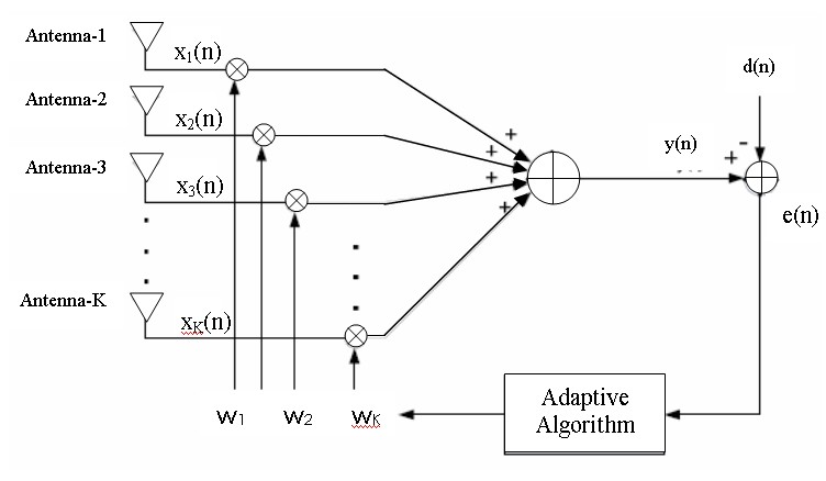
The purpose of beamforming is to form multiple beams towards desired users while nulling the interferers at the same time, through the adjustment of the beamformer’s weight vectors. Fig.1 shows a generic adaptive beamforming system which requires a reference signal. The signal x(n) received by multiple antenna elements is multiplied with the coefficients in a weight vector w (series of amplitude and phase coefficients) which adjust the phase and amplitude of the incoming signal accordingly. This weighted signal is summed up, resulting in the array output, y(n). An adaptive algorithm is then employed to minimize the error e(n) between a desired signal d(n) and the array output y(n). For the beamformer, the output at time n, y(n), is given by a linear combination of the data at the K sensors and can be expressed as [9]:
(1)
where w=[w1 … wK] and x(n)=[x1(n) … xK(n)], denotes Hermitian (complex conjugate) transpose. The weight vector w is a complex vector. The process of weighting these complex weights w1, …, wK adjusted their amplitudes and phases so that when added together they form the desired beam. Typically, the adaptive beamformer weights are computed in order to optimize the performance in terms of a certain criterion.
Most adaptive algorithms are derived by first setting a performance criterion and then generating a set of iterative equations to adjust the weights so that the performance criterion is met. Some of the most frequently used performance criteria include MMSE, maximum signal-to-interference-and-noise ratio (SINR), maximum likelihood (ML), minimum noise variance, minimum output power and maximum gain, etc. [10]. In order to obtain the optimum weight vector, one needs to know the second order statistics, which are usually unknown and change over time. Adaptive beamforming algorithms estimate them and update the weight vector over time. As the weights are iteratively adjusted, the performance of beamformer approaches the desired criterion. The algorithm is said to be converged when such a performance criterion is met.
Fig.1 A generic adaptive beamforming system
There are many types of adaptive beamforming algorithms that exist in the literature. Adaptive beamforming can separate signals transmitted on the same carrier frequency, provided that they are separated in the spatial domain. Most of the adaptive beamforming algorithms can be categorized under two classes according to whether training signal is used or not. These two classes are non-blind adaptive algorithm and blind adaptive algorithm. Non-blind adaptive beamforming algorithm uses a training signal d(n) to update its complex weight vector. This training signal is sent by the transmitter to the receiver during the training period. Beamformer in the receiver uses this information to compute new complex weight. LMS, NLMS, RLS and SMI algorithms are categorized as non-blind algorithm. Blind algorithms on the other hand do not need any training sequence to update its complex vector. Constant Modulus Algorithm (CMA) [11], Spectral self-Coherence Restoral (SCORE), and Decision Directed (DD) algorithms are examples of blind adaptive beamforming algorithms. These algorithms use some of the known properties of the desired signal. In blind algorithm, the goal is to retrieve the input signal by using output signal and possibly the statistical information for the input.
3. SMI-NCMA ADAPTIVE BEAMFORMING ALGORITHM
In this section, a new optimum SMI-NCMA algorithm is introduced for adaptive beamforming. In SMI-NCMA algorithm, the SMI algorithm is utilized to determine the optimum weight vectors assigned to each of the antenna elements of the array instead of arbitrary value before calculating the final weight vector. The weight is calculated only for the first few samples or for a small block of incoming data. The weight coefficients derived by SMI algorithm are set as initial coefficients and are updated by introducing NCMA algorithm. However, to improve the stability of the system and convergence speed, NCMA method is used instead of CMA (constant modulus algorithm). NCMA is CMA, but the step size is changed as the correlation matrix is changed to avoid unstable system. CMA supposes that the canal input signal is constant modulus. Every modification in the amplitude of the received signal is a canal distortion [12]. So, the weights are chosen to minimize envelope variance of the output signal.
In practice, the signals are not known and the signal environment frequently changes. Thus, adaptive processors must continually update the weight vector to meet the new requirements imposed by the varying conditions. Optimal weight vectors can be computed by obtaining an estimation of the covariance matrix R and the cross-correlation matrix r in a finite observation interval and then these estimates are used to obtain the desired vector.
The estimation of both R and r over a block size N2−N1 can be evaluated respectively as follows [5]:
(3)
(4)
where, N1 and N2 are the lower and upper limits of observation interval or window and n is the sample index. This limit is taken to be small, to ensure that the effect due to changes in the signal environment during block acquisition does not affect the performance of the algorithm. Also, large limit or block only means more matrix inversions, making the algorithm computationally intensive. The SMI algorithm requires the calculation of the inverse covariance matrix R and this incurs high computational complexity. The CMA algorithm avoids matrix inversion operation by using instantaneous gradient vector J to update the weight vector. If w(n) denotes the estimate of the weight vector at the nth iteration and J(n) is the mean square error, the next estimation of the weight vector for the (n+1)th iteration, w(n+1) is estimated according to the following simple recursion :
(5)
where µ is a small positive constant, called the step size whose value is between 0 and 1. The CMA algorithm is based on the steepest-descent method which recursively computes and updates the weight vector. From CMA [13] algorithm we know that:
(8)
(9)
In the CMA algorithm, Eq.(8) shows that the product vector µx(n)e*(n) at iteration n, applied to the weight vector w(n), is directly proportional to the input vector x(n). Therefore, the CMA algorithm experiences a gradient noise amplification problem when the input signal x(n) is large, i.e., the product vector µx(n)e*(n) is large. This is solved by normalization of the product vector at iteration n+1 with the square Euclidean norm of the input vector x(n) at iteration n [14]. The change of the weight vector is given as:
(9)
Which is subject to the constraint in order to minimize the square Euclidean norm in weight vector w(n+1) with respect to its previous value w(n). So:
(10)
where C(n) is the desired value (normalized to 1 for constant modulus envelope). The method of Lagrange multipliers is used to solve this constraint.
Optimization problem [details about Lagrange multipliers can be found in [14].
Using the complex constraint of Eq.(10) the conjugate Lagrange multiplier becomes:
Furthermore, substituting Eqs.(6) and (7) into Eq.(11) yields:
(12)
After equivalently manipulate, the weight vector can be written as:
(13)
As can be seen from Eq.(13), the algorithm reduces the step size µ to make the changes large. As a result, the step size µ varies adaptively by following the changes in the input signal level. This prevents the update weights from diverging and makes the algorithm more stable and faster converging than when a fixed step size is used. In addition, the NCMA algorithm is used as the MMSE method needs to cope with the large changes in the signal levels of mobile communication systems. By combining the above two algorithms, the new optimum SMI-NCMA algorithm update the weight vectors according to the following equations:
,
,
,
(14)
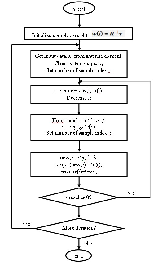
The final weight vector of the SMI-NCMA algorithm is estimated from Eq.(14). In the SMI-NCMA algorithm, advantages of both the block adaptive and sample by sample techniques are employed. In this algorithm, the initial weight vector is obtained by matrix inversion through SMI algorithm, only for the first few samples or for a small block of incoming data instead of arbitrary value before calculating the final weight vector. The final weight vector is updated by using the NCMA algorithm. The flowchart of the SMI-NCMA algorithm is shown in Fig.2.
The above description of the adaptive procedure based on the SMI-NCMA algorithm can be given as follows:
Step 1: Initial calculation of weight vector by matrix inversion (first few samples or small block of incoming data).
Step 2: Calculate the error and scale the input vector by the equations of the algorithm.
Step 3: Normalize the weight vector.
Step 4: Update the weight vector by final equation until convergence.
Fig. 2 Flow chart of the SMI-NCMA algorithm
4. Results and discussion
In this work, we consider a simple uniform linear array antenna of 8×1 element with half wavelength spacing between the elements, located at the base station to perform spatial filtering. Data sequences are generated using Binary Phase Shift Keying (BPSK) modulation and for the sake of simplicity the radio channel is assumed to be multipath free and non-dispersive with Additive White Gaussian Noise (AWGN). In the simulation, the angle of arrival of the desired user and the interferers are at 60°, 30° and 130° respectively. The signal to noise ratio (SNR) is set at 8 dB and the number of data bit length is 300. Error convergence plot, bit error rate, adaptive array pattern performances and weight convergence of the SMI-NCMA are evaluated and compared with typical NCMA algorithm; how use an orthogonal initial weight vector [15]; to demonstrate the merits of this new algorithm.
Figs.3 and 4 show the MSE plot or convergence plot for the NCMA and the SMI-NCMA algorithm respectively.
Fig.3 Mean square error plot for the NCMA algorithm
Fig.4 Mean square error plot for the SMI-NCMA algorithm
As shown in these figures, for the same adaptation size or iterations, the SMI-NCMA algorithm can achieve faster convergence than the typically NCMA algorithm. Also the NCMA algorithm starts to converge from the iteration number 200 whereas in the SMI-NCMA algorithm it starts to converge from the initial iteration. In this case, the NCMA error is almost 0.2591 and the SMI-NCMA error is almost 0.0568 at around 100 iterations.
Figs.5 and 6 present the linear and polar plot of the beampattern for the SMI-NCMA and NCMA algorithm respectively. These figures show that the SMI-NCMA generates deeper nulls of about −200 dB and NCMA generates nulls between -50 dB and -80 dB towards the interferers, giving big improvements for the SMI-NCMA algorithm in interference suppression with respect to NCMA algorithm. Both algorithms have their main beam pointed to the desired user direction. The ratio of main lobe to the first side lobe is 43 dB and 30 dB for SMI NCMA and NCMA respectively.
Fig.5 Comparison of linear beampattern of SMI-CMA and NCMA algorithms
Fig.6 Comparison of polar beampattern of SMI-NCMA and NCMA algorithms
Co–Channel Interference (CCI) is a major factor that limits the capacity of a cellular system. To increase the capacity of a cellular system, frequency is reused, i.e., a frequency band is used in two different cells belonging to different clusters, which are sufficiently separated so that they do not interfere significantly with each other. The BER performances with respect to the number of CCI of the two algorithms are presented in Fig.7. As can be seen from the figure, for CCI equal to 10, BER for the NCMA and the SMI-NCMA are 4.53×10⁻² and 3.6×10⁻² respectively. Fig.7 also shows that BER increases as the number of interferer increases for both algorithms and that SMI-NCMA provide about 20.5% BER improvement at CCI equal to 10 over that of NCMA algorithm.
Fig.7 BER performance of the SMI-NCMA and NCMA algorithms with varying CCI
Fig.8 shows the comparison of BER with 8-element antenna array for SMI-NCMA and NCMA algorithms. The BER performance is greatly improved in the SMI-NCMA algorithm compared to the NCMA algorithm. The BER rate of the SMI-NCMA and NCMA algorithm are 1.68×10⁻² and 7.67×10⁻² respectively. The reduction of the BER for SMI-NCMA is 78% compared to NCMA algorithm.
Fig.8 Performance of BER with 8-element antenna array for SMI-NCMA and NCMA algorithms
The magnitude of the complex weights plotted against the number of samples for each antenna element is presented in Fig.9 by using NCMA algorithm. The convergence of the weights to their optimum values for NCMA algorithm is shown in the figure. The complex weights at the iteration 1200 for NCMA algorithm are as follows:
Table 1 : Magnitude and phase of the complex weights for the NCMA algorithm
Fig.9 Weight convergence plot of the first 8 antenna elements for SMI-NCMA algorithm
Fig.10 shows the magnitude of the complex weights plotted against the number of samples for each antenna element by using SMI-NCMA algorithm. It is evident that the weight values converge to their optimum values for SMI-NCMA algorithm.
The complex weights at the iteration 1200 for SMI-NCMA algorithm are as follows:
Table 2 : Magnitude and phase of the complex weights for the SMI-NCMA algorithm
Fig.10 Weight convergence plot of the first 8 antenna elements for SMI-NCMA algorithm
As can be observed from Fig.10, the SMI-NCMA starts adaptation to optimum weights from the initial weight vector values. On the contrary, NCMA algorithm has to converge from the arbitrary weight values (in this case 1) to the optimum weight values. However, before it converges to its optimum values, the interfering directions will change; consequently more iterations are needed to converge.
5. CONCLUSION
In this paper, we introduced a novel and less complex adaptive beamforming algorithm, the “SMINCMA”, for smart antenna system. SMI-NCMA combines the SMI and NCMA algorithms to improve the convergence speed with small BER. In this algorithm individual good aspects of both the sample by sample and block adaptive algorithms are employed. SMI-NCMA computes the optimal weight vector based on the SMI algorithm and updates the weight vector by NCMA algorithm. Simulation results showed that the SMI-NCMA algorithm provides remarkable improvements in terms of interference suppression, convergence rate and BER performance over that of classical NCMA algorithms. With respect to NCMA, SMI-NCMA provides: (1) big improvements in interference suppression, (2) 13 dB gain enhancement, (3) convergence from the initial iteration (whereas NCMA convergence from the iteration number 200), and (4) 20.5% BER improvements at CCI equal to 10. The reduction of the BER for SMI-NCMA is 78% compared to NCMA algorithm in the case of 8-element antenna array.
References
S. Denno, T. Ohira, "M-CMA for digital signal processing adaptive antennas with microwave beamforming", IEEE Aerospace Conference Proceedings, vol.5, N°4, Page(s): 179 – 187. 2000.
S. Chen, N.N. Ahmad, L. Hanzo, “Adaptive minimum bit-error rate beamforming”. IEEE Transactions on Wireless Communications, Vol. 4, N° 2, pp.341-348, 2005.
H. Krim, M. Viberg, “Two decades of array signal processing research: the parametric approach”, IEEE Signal Processing Magazine, 1996, Vol13, N°4, pp.67-94.
J.C. Liberti, T.S Rappapoert, Smart Antenna for Wireless Communications Is-95 and Third Generation CDMA Applications. Prentice-Hall PTR, New Jersey, 2002.
M.W. Ganz, R.L. Moses, S.L. Wilson, “Convergence of the SMI and the diagonally loaded SMI algorithms with weak interference (adaptive array)”. IEEE Transaction, Antennas Propagation, Vol.38, N°3, pp.394-399. 1990.
D. Liu,; L. Tong, "An analysis of CMA for array signal processing", IEEE International Symposium on Information Theory, Volume5, Issue 4, Page(s):181-192. 1998
L.J. Griffiths, “A simple adaptive algorithm for real-time processing in antenna arrays”, IEEE Signal Processing Magazine, 1969, Vol.57, pp.1696-1704.
B. Widrow, P.E. Mantey, L.J. Griffiths, B.B. Goode, Adaptive antenna systems, IEEE Signal Processing Magazine, 1967, Vol55, pp.2143-2159.
A. El-Zooghby, "Smart Antenna Engineering "Artech House Mobile Communications Library, 2005.
J. Litva, T.LO. Kwok-Yeung. Digital Beamforming in Wireless Communications, Artech House Boston, 1996.
J.R Treichler, B.G Agee, “A new approach to multipath correction of constant modulus signals”, IEEE Transaction on Acoustics, Speech and Signal Processing, Vol. ASSP-31, April 1983.
B.G. AGEE, “Convergent behavior of modulus- restoring adaptive arrays in Gaussian interference environments”, Proc. of the Asilomar Conf. on Signals, Systems, and Computers, Decp. 818-822. 1988.
J. LI, P. Stoica, Robust Adaptive Beamforming, A John Wiley & sons, inc.2005.
S. Haykin, Adaptive Filter Theory (3rd Ed.). Prentice Hall, New York. 1996.
T.E. BIEDKA, “A comparison of initialization schemes for blind adaptive beamforming”, IEEE International Conference on Acoustics and Signal Processing, Vol. 3, p.1665-1668. 1998.