UDC 621.373, 519.622

ACCURACY ESTIMATION OF THE NUMERICAL METHODS  OF THE ANALYSIS OF THE RELAXATION OSCILLATOR

 

A. M. Pilipenko, V. N. Biryukov

Southern Federal University, Nekrasovsky 44, Taganrog 347922, Russia

 

The paper is received on November 6, 2013

 

Abstract. In the paper the modern numerical methods for solving ordinary differential equations are testing. These methods are widely applied in simulators of RF circuits. As a test problem the relaxation oscillator’s differential equation with arbitrary polygonal nonlinearity was selected. An estimation of accuracy of numerical methods is received in the case of simulation of the relaxation oscillator. It is shown that the error of solution is determined by the methodological error and random errors caused by 1) an error of synchronization of the numerical solutions with the period of oscillation, 2) changes in the current step. It is shown that the random error of the RADAU method far exceeds the same error of the BDF method.

Keywords: numerical methods, nonlinear differential equations, relaxation oscillator, error analysis.

 

1. Introduction

Computer modeling of RF circuits and devices in the time domain consists in the numerical solution of systems of ordinary differential equations (ODE). In modern packages of circuit design and automation of engineering calculations, a large number of numerical methods for solving ODE are implemented. The main criteria for the effectiveness of numerical methods are their computational complexity and the accuracy of the solutions obtained. The accuracy of computer simulation quantitatively characterizes the degree of deviation of the simulation results from the exact results. For a theoretical assessment of the accuracy of numerical methods for solving ODE linear ODEs are used as a rule, for which an exact solution is known. Real radio engineering devices are described by nonlinear ODEs, therefore, assessing the accuracy of their numerical analysis is a quite complicated task.

In [1], a study was carried out of the accuracy of modern numerical methods in the analysis of harmonic oscillation generators. This article is a continuation of [1] as applied to another class of self-oscillating circuits — relaxation oscillation generators. The aim of this work is to assess the accuracy of modern numerical methods for solving ODEs in the simulation of relaxation generators.

The choice of the problem of analysis of the generator of relaxation oscillations as a test is due to the following reasons. Firstly, a relaxation generator is an integral part of many electronic devices, such as functional generators, radio measuring devices, counters, timers, devices that initiate measurements or technological processes [2]. Secondly, the task of numerically analyzing a relaxation generator in the time domain is one of the most difficult for computer modeling, since the ODEs describing a self-oscillator is often both oscillatory and stiff [3]. Thus, an assessment of the accuracy of the numerical analysis of the relaxation generator is necessary to select the most effective method for modeling self-oscillating systems with varying degrees of stiffness.

2. Model of relaxation generator

Relaxation oscillations occur in nonlinear electrical circuits that do not have frequency selectivity. The simplest circuit model of a relaxation generator can be presented as well as a model of a harmonic oscillation generator — in the form of a parallel connection of three elements — a linear capacitance C and an inductance L and a nonlinear resistive element whose differential resistance (conductivity) can change its sign [1].

The mathematical model of the relaxation generator (self-oscillator equation) has the form of a nonlinear differential equation of the second order:

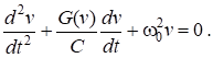                                      (1)
 

where v is the voltage at the generator output,   is the resonant frequency of the LC circuit, G(v) = di(v) / dv is the differential conductivity of the nonlinear element, i (v) is the I – V characteristic of the nonlinear element.

 

If the differential conductivity G (v) in the initial portion of the I – V characteristic near zero takes a negative value, then self-oscillations occur in the LC circuit. When approximating the I – V characteristic of a nonlinear element by a third-degree polynomial i(v) = a₁v + a₃v³ (a₁<0, a₃ > 0), equation (1) is called the Van der Pol equation and its analytical solutions are known for the steady state. Unfortunately, the solution cannot be obtained explicitly, and there are only standard numerical solutions specially calculated with high accuracy for some parameters of the equation [4].

To obtain an analytical solution of the oscillator equation in the steady state, one can use the technique proposed in [5]. This technique consists in applying a piecewise linear approximation of the I – V characteristic of a nonlinear element. This approach allows us to determine the stationary solution of the oscillator equation with relative error about 10^-16.

The relaxation generator is characterized by significant losses that can be estimated by damping factor

where  is the characteristic conductivity of the LC-circuit, G₁ is the differential conductivity of a nonlinear element at di / dv > 0.

In the case of significant losses, d > 2 and the solution of a linear homogeneous second-order differential equation is described by the sum of two exponential functions. Thus, when using a symmetric piecewise linear function to approximate the I – V characteristic of a nonlinear element, the analytical expression for the voltage at the output of the relaxation generator in the steady state has the form [1]

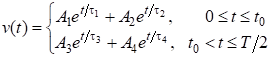                             (2)
 

where  A₁,  A₂,  A₃,  A₄ are the integration constants; t₀ is the point in time at which the conductivity of the nonlinear element changes sign; T is the period of oscillation; ; are time constants of the oscillator at G (v) = G₀ < 0 and G (v) = G₁ > 0, respectively; d_0,1 = | G_.0,1 / 2C |

Fig. 1 shows the exact stationary solutions of the oscillator equation obtained using expression (2) for two different attenuation values d = 4 (solid line) and d = 100 (dashed line), the values of the remaining parameters of the oscillator were set as follows: L = 1 H, C = 1 F, G₀ = - 4 S.

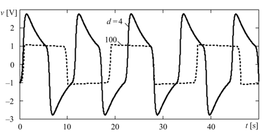
Fig. 1. Exact stationary solutions of the oscillator equation.

 

 

It should be noted that for d = 4, the self-oscillator model (1) can be considered weakly stiff, since in this case the stiffness coefficient is equal to the ratio of the maximum and minimum self-generator time constants η = τ_max / τ_min ≈ 10 > 1. For d = 100, the model (1) is stiff, since in this case η ≈ 10⁴ >> 1.

The obtained analytical solutions make it possible to estimate the main oscillation parameters at the output of the oscillator with a relative accuracy of about 10 ^-14. Table 1 shows the exact amplitudes A_m0 and the exact frequencies f_m0 of the relaxation oscillations shown in Fig. 1.

Table 1

 

 

3. Numerical solution of the oscillator equation

In this paper, we estimated the accuracy of modeling the relaxation generator in the time domain using three numerical methods for solving ODE: the trapezoid (TR), BDF, and RADAU5 methods. A detailed description of these methods is given in [6, 7]. The choice for the numerical analysis of the TR and BDF methods is explained by the fact that they are the main methods for the analysis of transients in electronic simulators. The RADAU5 method is one of the most promising methods of the Runge-Kutta type for solving stiff problems [7]. It should be noted that the RADAU5 method is three-stage, therefore, its application is reduced to solving a system of algebraic equations, the order of which is three times the order of the ODE of a given circuit. The TR and BDF methods are one-stage, thus, the computational complexity of these methods, which determines the computer time and RAM to obtain a solution, is minimal. Multistage methods have increased L-stability and are recommended for solving problems of high stiffness [8, 9].

To assess the accuracy of the above numerical methods, we apply the technique proposed in [10] and based on the analysis of the accuracy of the assessment of the main parameters of the generated oscillation - frequency and amplitude. The current relative errors in the estimation of frequency and amplitude are respectively determined using the following relations

,   ,

 

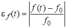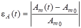where f(t) and A_m(t) are estimations of the frequency and amplitude of the generated oscillation obtained from solving equation (1) by numerical methods.

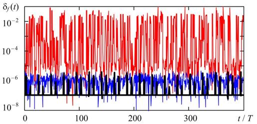
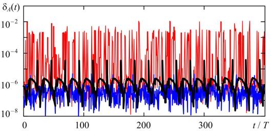
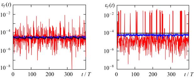
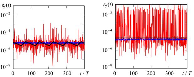
Figures 2 and 3 show the time diagrams of the relative errors in estimating the frequency and amplitude of the stationary oscillations of the relaxation generator for various attenuation and, accordingly, the stiffness of the oscillatory system (see table 1). The equation (1) was solved by the numerical methods listed above for a given maximum step h_max = T/1000 and the maximum acceptable relative error TOL = 10^-5. To estimate the oscillation frequency, we used linear interpolation of the numerical solution at the points of sign change v(t), and to estimate the amplitude, we used the quadratic interpolation at points of local extrema. The observation interval is selected corresponding to the stationary generation mode.

Fig. 2 and Fig> 3 show the process parameters f_m(t) and A_m(t) vary significantly from one period to another. For a quantitative description of the results obtained in table 2 shows the average values of the relative errors in estimating the frequency and amplitude of oscillations (m_εω and m_εA, respectively) and standard deviations (RMS) of the relative errors in estimating the frequency and amplitude of oscillations (σ_εω and σ_εA, respectively).

 

 

  

(a)                                                                                                      (b)

 

Fig. 2. Current relative errors in estimating the frequency of relaxation oscillations using the TR, BDF, and RADAU5 methods
with h_max = T/1000, TOL = 10^-5, and various stiffness of the oscillator model. η = 10 (a) and η = 10⁴ (b).

 

 

 

 

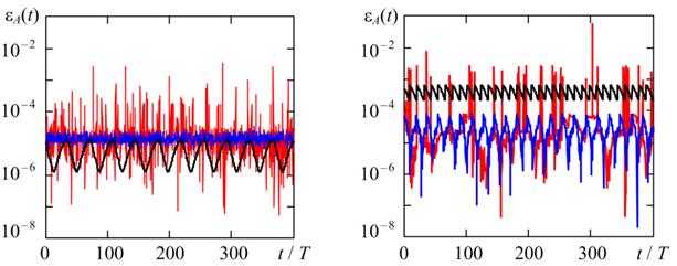
 (a)                                                                                                     (b)

 

Fig. 3. Current relative errors in estimating the amplitude of relaxation oscillations as in the case of Fig. 2

 

Table 2

 

The results of the numerical analysis shown in Fig. 2, Fig. 3 and in Table 2, show that the RADAU5 method, as a rule, has the largest values of relative errors both in estimating the frequency and in assessing the amplitude of relaxation oscillations, regardless of the stiffness of the problem. In addition, the current error values for the RADAU5 method can be one or two orders of magnitude higher than the similar errors of the BDF and TR methods. This effect is especially expressed when estimating the frequency in the case of high stiffness of the problem (see Fig. 2, b). In the case of weak stiffness of equation (1) (η = 10), the relative errors for the BDF and TR methods are of the same order of magnitude.

At high stiffness (η = 10 ⁴), the current errors ε_f (t) and ε_A(t) turn out to be the smallest for the BDF method, and the average value of the error in estimating the amplitude for the BDF method is approximately 15 times lower than the corresponding value for the TR method. It should be noted that the errors of the BDF method depend most weakly on the stiffness of the problem in comparison with the errors of the other methods considered. As can be seen from Table 2, with an increase in the stiffness of the problem by a factor of 10³, the relative errors for the BDF method increase no more than 4.5 times, while for the TR and RADAU5 methods they can increase more than 50 times.

It follows from Fig. 2 and Fig. 3 that for the TR and BDF methods, the effect of synchronization of the error with the period of generated oscillations can be observed. In this case, the current errors are, as a rule, periodic in nature, and the period of change in errors is a multiple of the period of generated oscillations. In addition to the “synchronization error”, the second random component is the error observed in the BDF and RADAU5 methods, caused by the step change algorithm in the solution process. To verify the correctness of the implemented accuracy assessment methodology demonstrated in Fig. 4 and Fig. 5 shows the current relative errors in estimating the frequency and amplitude of relaxation oscillations using the TR, BDF, and RADAU5 methods with a 2-fold decrease in h_max and a 4-fold TOL as compared to the case shown in Fig. 2 and Fig. 3.

 

 

 

 

 

 

(a)                                                                                                 (b)

 

Fig. 4. Current relative errors of frequency estimation by the considered methods for different stiffness
η = 10 (a) and η = 10⁴ (b); h_max = T/2000, TOL = 0.25 10 ^-5.

 

 

 

 

 

 

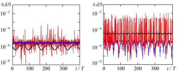
(a)                                                                                                 (b)

 

Fig. 5. Current relative errors of amplitude estimation by the considered methods for different stiffnes
 η = 10 (a) and η = 10⁴ (b); h_max = T/2000, TOL = 0.25 10 ^-5.

 

From a comparative analysis of the errors given in Figs 2, 3 and in Figs 4, 5 it is seen that with a decrease in TOL by 4 times, the average values and standard deviations of the errors of the TR and BDF methods also decrease about 4 times, and the synchronization effect weakens. For the RADAU5 method, errors are reduced only in the case of a weakly stiff problem, and in the case of a stiff problem, a significant increase in the current errors ε_f (t) and ε_A (t) is observed. Such an effect for the RADAU5 method can be explained by a sharp increase in the rounding error with a decrease in the solution step and the effect of the method’s dense output. The rounding error of the RADAU5 method increases due to poor conditioning of the corresponding system of algebraic equations, the order of which is three times the order of the original system of ODEs [7].

4. Estimation of the random component of the numerical error analysis in the absence of an exact solution

It should be noted that the analysis of the error of the numerical solution can be carried out partially even in the case when the exact solution is absent. The accuracy can be estimated by calculating the relative deviations of the values of the oscillation parameters obtained in the current and subsequent periods of the decision:

;

In the general case, increments of errors on adjacent periods should be less than or equal to the optional error. However, as shown in Fig. 6 and Fig. 7, the dependences δ_f (t) and δ_A(t) obtained by solving equation (1) by the same methods and at the same values of h_max and TOL as the dependences ε_f (t) and ε_A (t) in Fig. 4b and Fig. 5b are not always small. Thus, excess solution noise can be detected without determining the exact values of the process parameters.

 

 

 

  

 

Fig. 6. The dependences δ_f (t) obtained by the using the TR, BDF, and RADAU5 methods at h_max = T/2000, TOL = 0.25 10 ^{- 5}, and η = 10⁴. 

 

 

 

 

Fig. 7. The dependences δ_A (t) obtained by the using the TR, BDF, and RADAU5 methods at h_max = T/2000, TOL = 0.25 10 ^{- 5}, and η = 10⁴.

 

5. Discussion

Evaluation of the accuracy of solving a particular problem by local or even interval (global) error does not give a general idea of the accuracy of the analysis of a numerically modeled process. Often, to prove the suitability (or unsuitability) of a method, a schedule for solving a one-dimensional or two-dimensional problem is given [7, 9]. The lack of a quantitative assessment of the quality of modeling of the investigated process leads to attempts to supplement the concept of "error of solution" with the concept of "reliability of the solution".

In the present work (and in [1]), the estimation of the error of the solution was carried out according to the parameters of the investigated periodic process. This approach allows us to replace the huge data array of current errors with a much more compact and visible one, which in some cases allows us to perform a more detailed analysis of the error structure that is not available to graphical methods. In the case under consideration, the RADAU5 method revealed a significant component of the error caused, apparently, by the imperfection of the algorithms for automatic step selection and / or dense output. The corresponding Gear algorithm turned out to be, on the contrary, very efficient. Evaluation of the error of the solution by the parameters of the stationary process allows us to detect random error components associated with the synchronization of the solution with the step and the imperfection of the step selection algorithm for any problem with a periodic solution without determining the exact solution.

Summary

The estimation of the accuracy of the numerical analysis of the relaxation generator complements the known theoretical and experimental estimates of the properties of numerical methods for solving differential equations for oscillating systems given in [1, 10, 11]. The accuracy of the methods was controlled not by the error in determining the variable, but by the errors in determining the main parameters of the stationary process - the frequency and magnitude of the oscillation. As a test problem, the analysis of a self-oscillator is considered, in which the I – V characteristic of a nonlinear element is approximated by a piecewise-linear function, which allows one to obtain an exact stationary solution and its main parameters necessary for estimating the errors of the tested numerical methods.

The results of testing of the numerical methods obtained in this paper allow us to substantiate the choice of one or another method for obtaining reliable and most accurate simulation results for self-oscillating systems with varying degrees of stiffness. In addition, in this paper, a method for evaluating the accuracy of the numerical analysis of nonlinear oscillatory systems in the absence of an exact solution is proposed and justified.

Acknowledgment

This work was supported by a scholarship of the President of the Russian Federation for young scientists and graduate students (SP-398.2012.5).

 

References

1.     Pilipenko A. M.,   Biryukov V. N.   Investigation of modern numerical analysis methods of self-oscillatory circuits efficiency. Journal of Radio Electronics. 2013. No 8. URL:   http://jre.cplire.ru/jre/aug13/9/text_e.pdf

2.     Horowitz P., Hill W. The Art of Electronics. Cambridge University Press, 2015.

3.     Pilipenko A. M., Biryukov V. N. Hybrid Methods for Solution of Ordinary Differential Equations of Stiff and/or Oscillating Circuits. Radio Engineering. 2011. No 1. pp. 11-15 (in Russian).

4.     Guzhev D. S., Kalitkin N. N. Burgers equation - a test for numerical methods. Mathematical modeling. 1995. Vol. 7. No 4, pp. 99 – 127 (in Russian).

5.     Biryukov V. N., Gatko L. E. Exact stationary solution of the oscillator nonlinear differential equation. Nonlinear World. 2012. Vol. 10. No. 9. pp. 613-616 (in Russian).

6.     Hairer E., Nørsett S. P., Wanner G. Solving Ordinary Differential Equations I. Nonstiff Problems. Springer, 1993.

7.     Hairer E., Wanner G. Solving Ordinary Differential Equations II. Stiff and Differential-Algebraic Problems. Springer, 1996.

8.     Kalitkin N. N. Numerical methods of solution of stiff systems, Mathematical modeling. 1995. Vol. 7. No. 5, pp. 8–11 (in Russian).

9.     Maffezzoni P., Codecasa L., D’Amore D. Time-domain simulation of nonlinear circuits through implicit Runge-Kutta methods. IEEE Transactions. Circuits and Systems. 2007. Vol. 54. No. 2, pp. 391 – 400.

10.  Biryukov, V.N., Pilipenko, A.M.; Kovtun, D.G. Estimation of the Numerical Methods' Accuracy of Oscillating Differential Equations Analysis in Time-Domain Radioengineering. 2011. No. 9. pp.104-107.

11. Biryukov V. N., Pilipenko A. M. An Approach to Estimate the Error of Oscillator Time-Domain Analysis. Proceedings of IEEE East-West Design and Test Symposium (EWDTS'2013). 2013. pp. 223-226.