


Next: The Exact Analytical Expression
Up: Approximation of distribution function
Previous: Introduction
Consider a  -element antenna array with arbitrary
locations of sensors. The -dimensional input signal
-element antenna array with arbitrary
locations of sensors. The -dimensional input signal  is assumed to be complex random Gaussian vector. We suppose
that
is assumed to be complex random Gaussian vector. We suppose
that  samples of the signal
 are
statistically independent and identically distributed
(i.i.d.) zero-mean random vectors with spatial covariance
matrix
are
statistically independent and identically distributed
(i.i.d.) zero-mean random vectors with spatial covariance
matrix  . By reviewing of non-singular case, let us
suppose that the sample size is greater than the number
of the antenna elements
. By reviewing of non-singular case, let us
suppose that the sample size is greater than the number
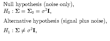
of the antenna elements  . The problem of detection
of some spatially correlated useful signal by the antenna
array is formulated as a classical two-hypothesis
alternative:
. The problem of detection
of some spatially correlated useful signal by the antenna
array is formulated as a classical two-hypothesis
alternative:
|
|
|
|
(1) |
where  is the identity matrix, and
  is the
a-priori unknown noise power.
is the
a-priori unknown noise power.
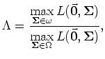
For the problem considered herein, the GLR test-statistic is given by
|
|
|
|
(2) |
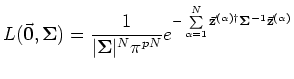
where
|
|
|
|
(3) |
is the likelihood function for complex variables,  is the
parameter sub-region corresponding to the null hypothesis
is the
parameter sub-region corresponding to the null hypothesis  in
the parameter space
in
the parameter space  ,
,  is the determinant of a
matrix and the superscript
is the determinant of a
matrix and the superscript  represents the transpose
conjugate or Hermitian operator. Note that the
test-statistic obtained accordingly with (2)
can accept values only in interval [0,1].
represents the transpose
conjugate or Hermitian operator. Note that the
test-statistic obtained accordingly with (2)
can accept values only in interval [0,1].
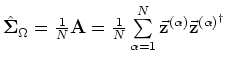
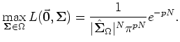
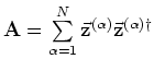
It can be shown [1] that maximum value of the
GLR (2) denominator is achieved by using
maximum likelihood estimation
 of the
covariance matrix :
of the
covariance matrix :
and this value is equal to
|
|
|
|
(4) |
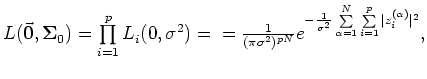
The maximum of the GLR (2) numerator should be
obtained in parameter sub-region ( ) corresponding to the null hypothesis (1).
If hypothesis is true, the likelihood function is given as:
) corresponding to the null hypothesis (1).
If hypothesis is true, the likelihood function is given as:
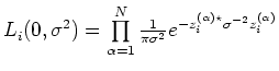
where
 is the
likelihood function of the signal from the
is the
likelihood function of the signal from the  -th sensor.
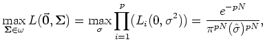
From the last expression for the likelihood function the
maximum value of the GLR (2) numerator is
easily obtained
|
|
|
|
(5) |
and this maximum is achieved by using maximum likelihood
estimation
 of the variance
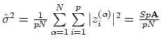
where
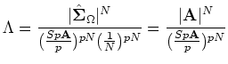
Taking into account the
expressions (4), (5) the GLR
test-statistic (2) for the problem
(1) can be represented as:
|
|
|
|
(6) |
The rejection region of the hypothesis is determined by
the inequality  , where
  is the test-statistic
threshold only dependent upon the given false alarm probability level
is the test-statistic
threshold only dependent upon the given false alarm probability level
 .
.
Next: The Exact Analytical Expression
Up: Approximation of distribution function
Previous: Introduction