|
|
"JOURNAL OF
RADIOELECTRONICS" N 1, 2002 |
|
Cyclotron and Synchronous Oscillations and Waves of
the Electron Beam
General Relations
Vladimir A. Vanke,
e-mail: vanke@mesps.phys.msu.su
Moscow State
University
Received 05 January 2002
General relations of the cyclotron and
synchronous oscillations and
waves of the electron beam are discussed in a
form of short review.
I.
Introduction
III.
Kinematics Analysis
IV.
Transverse (Cyclotron
and Synchronous) Waves of the Electron Beam
V.
Kinetic Powers of
Transverse Waves
VI.
Numerical
Simulation and Helix-Type Discretization of the Injecting Electron Beam
VII.
Discussion
VIII.
Selected
Bibliography
I. Introduction
Development of modern microwave communication, radio and radar facilities
places additional stringent requirements upon the different microwave
devices.
During last several decades
mainly in Russia active and successful work is being carried on to create new
electron beam microwave devices based on cyclotron and synchronous waves use [1-16] and complying
with the present-day requirements.
The operation of these devices is based on the principles of transverse
grouping of the electron beam in the longitudinal magnetic field. In contrast
to conventional longitudinal grouping of electrons into dense bunches, this
principle employs the Lorenz force as an elastic force and leads to spatial
distortion of the electric beam without electron bunches being formed. In this
way it is possible to considerably overcome the fundamental restrictions, which
are characteristic of longitudinal grouping devices (both vacuum and
solid-state ones) and are associated with non-linear influence of the space
charge fields upon the process of the input signal amplification, thereby laying
the basis for developing new microwave devices with essentially improved
characteristics [6,9,12-16].
Author’s experience in discussions of these principles both with domestic and
foreign specialists has disclosed the expediency of the preparation of this
article.
II. A Simple Beam Model
Consider the motion of electrons in crossed electric and magnetic fields having
the form
Let us represent the beam as an aggregate of flat discs of infinitesimally
small thickness, moving along the z-axis with constant velocity ![]() . If the transverse dimensions of the discs and its displacements
from the unperturbed position are small in comparison with wavelength, then the
coupling between the discs, due to the longitudinal space charge, is also
insignificant and can be neglected. The problem is reduced to an analysis of
the transverse oscillation of the individual discs [17].
. If the transverse dimensions of the discs and its displacements
from the unperturbed position are small in comparison with wavelength, then the
coupling between the discs, due to the longitudinal space charge, is also
insignificant and can be neglected. The problem is reduced to an analysis of
the transverse oscillation of the individual discs [17].
Let the behavior of the individual (i-th) electron (![]() in Fig 2.1) be
characterized by a complex coordinate
in Fig 2.1) be
characterized by a complex coordinate ![]() (
(![]() ), let the coordinate of the mass center (C in Fig.2.1)
), let the coordinate of the mass center (C in Fig.2.1)
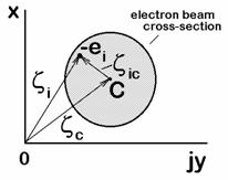
Fig. 2.1
Electron beam cross-section
of the disc be  , where
 ![]() is the number of electrons
in the disc. Then the orbits of the individual electron relative to
the mass center of the disc are described by the coordinates
is the number of electrons
in the disc. Then the orbits of the individual electron relative to
the mass center of the disc are described by the coordinates ![]() . The equation of the transverse motion in terms of the
variables
. The equation of the transverse motion in terms of the
variables ![]() assumes, in complex
notation, the forms
assumes, in complex
notation, the forms

where ![]() are the angular cyclotron frequency and the specific
charge of the electron, respectively;
are the angular cyclotron frequency and the specific
charge of the electron, respectively; ![]() ,
, ![]() are the external electric forces acting on the electrons
numbered by “i” and “k”.
are the external electric forces acting on the electrons
numbered by “i” and “k”.
Principal
interest attaches to the last two equations. The first of them characterized
the motion of the mass center of the cross section of the beam, and
consequently, describes the behavior of the signal and of the noise of the beam
as a whole. While the second is important in the investigations of the internal
structure of the beam (expansion of the thermal orbits, their balancing, etc).
The analytical solution of the problem with Coulomb sum in Eqs. (2.2) and (2.4), entails
considerable difficulties. Appreciable simplification can be obtained for a model
of a round uniformly charged cylindrical beam, if one uses the approximation

(where ![]() is
the plasma frequency),
is
the plasma frequency),
which in a number of cases makes it
possible to describe correctly the actual physical processes in the system [17,18].
It
is important to emphasize that in the cases when the function![]() depends linearly on the transverse coordinates and their
derivations, or else entirely independent of them, the equation of motion (2.3) for the mass
center of the discs coincides with the equation of motion for a single electron
without allowance for the Coulomb interaction and given by
depends linearly on the transverse coordinates and their
derivations, or else entirely independent of them, the equation of motion (2.3) for the mass
center of the discs coincides with the equation of motion for a single electron
without allowance for the Coulomb interaction and given by
where ![]() is
the external electric force acting on an electron placed at the mass center of
the disc.
is
the external electric force acting on an electron placed at the mass center of
the disc.
III. Kinematics Analysis
Let us introduce the transit angle![]() , and then
omitting
, and then
omitting ![]() subscripts, we can write
the equation of motion of one electron
subscripts, we can write
the equation of motion of one electron
 .
(3.1)
.
(3.1)
In the simplest case ![]() , i.e. when electric fields are absent, the solution has the
form
, i.e. when electric fields are absent, the solution has the
form
Now let ![]() using
the constant variation method, the solution will be sought in the form
using
the constant variation method, the solution will be sought in the form
then
 .
(3.4)
.
(3.4)
Since instead of one variable![]() , two new variables -
, two new variables -![]() are introduced, it is necessary to impose an additional
condition to connect these variables. A suitable condition for this
purpose is [19]
are introduced, it is necessary to impose an additional
condition to connect these variables. A suitable condition for this
purpose is [19]
then
 .
(3.7)
.
(3.7)
Substituting (3.6) and (3.7) in (3.1) and using (3.5), we obtain the
system of the first-order differential equations for the synchronous ![]() and cyclotron
and cyclotron ![]() radiuses
(see Fig. 3.1)
radiuses
(see Fig. 3.1)
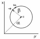
Fig. 3.1
Synchronous (a) and
cyclotron (b)
radiuses of an electron (-e) motion
Thus, the change in the cyclotron
orbit radius and the position of the orbit center with respect to the origin
are described separately, which provides an additional illustrative
representation and clarity of physical interpretation of the processes involved
in the interaction of the electron with external fields.
In the general case
![]() .
(3.9)
.
(3.9)
However, the solution of the
system (3.8) can
be simplified significantly in two extreme cases:
1. Short lenses, when the transit angle inside the
interaction region is small (Q<<1), and consequently,
in the right-hand parts of the system of equations (3.8) one can take
2. Adiabatic action of the fields on the electron
motion, when relative changes in a and b are
small during the oscillation period. In this case it is possible to use the
method of averaging by a rapidly oscillating phase, i.e. one can write

Calculating the integrals in the right-hand parts of these equations the values
of a and b should be taken constant [19].
The solution obtained from the smoothed (averaged) equations (3.11) takes into
account only effects of first order of smallness. In those cases when this does
not suffice, it is necessary to apply to Eq. (3.1) the asymptotic
methods of the theory of nonlinear oscillations [20].
For many issues of the theory of cyclotron-wave devices, the structure of the
external forces is such that Eq. (3.1) can be written
in a bit more convenient form
 ,
(3.12)
,
(3.12)
where
![]() ,
, ![]() is the angular frequency of the resonant harmonic or
subharmonic of the external force,
is the angular frequency of the resonant harmonic or
subharmonic of the external force, ![]() is the
relative difference between the natural frequency of the system
is the
relative difference between the natural frequency of the system ![]() and
and ![]() , the value of the parameter
, the value of the parameter ![]() is chosen such that it characterized the intensity of the
external forces.
is chosen such that it characterized the intensity of the
external forces.
The character of the action of the field on the beam is most frequently
adiabatic in practice, i.e., the values of a and b change little under the influence of this field within the
period of the fundamental motion. This is mathematically reflected in the
smallness of the parameter ![]() . In this of
a resonance adiabatic field
. In this of
a resonance adiabatic field ![]() a solution can be sought
for the n-th approximation, unlike (3.3), in the form
a solution can be sought
for the n-th approximation, unlike (3.3), in the form

where
the functions ![]() take into account all
arbitrary harmonics in
take into account all
arbitrary harmonics in ![]() , with the exception of the
zero-th and the first (the latter requirement is essentially a supplement
condition similar to (3.5)).
, with the exception of the
zero-th and the first (the latter requirement is essentially a supplement
condition similar to (3.5)).
The abbreviated equations are sought in this case also in the form of an
expansion in powers of the small parameter ![]()

Substituting (3.13) and (3.14) in the
initial equation (3.12)
and equating the terms of equal powers of ![]() in the
right and left sides of (3.12), we obtain
for the first two approximations
in the
right and left sides of (3.12), we obtain
for the first two approximations
![]() ,
, ![]() ,
(3.15)
,
(3.15)
where
 .
(3.16)
.
(3.16)
Accordingly
![]() ,
(3.17)
,
(3.17)
![]() ,
(3.18)
,
(3.18)
where

 ,
(3.20)
,
(3.20)
 .
(3.21)
.
(3.21)
 ,
(3.22)
,
(3.22)
 .
(3.23)
.
(3.23)
The first approximation of the asymptotic method does not differ from averaging
method [19]. The
second and succeeding approximations refine the first and make it possible to
take into account successively in the solution [19] the small high
frequency vibrations (harmonics of the signal and pump, combination
frequencies, etc.), which appear against the background of the fundamental
motion of the system [6].
IV. Transverse (Cyclotron and
Synchronous) Waves
of the Electron Beam
In the simplest case when external fields have the form (2.1), the equations
of motion of an electron are given by
 ,
(4.1)
,
(4.1)
 ,
, ![]() ,
, ![]() .
(4.2)
.
(4.2)
Now let us assume z and t to be
independent variables, thereby making a transition from the description of the
motion of one electron to the description of the motion of a filamentary
electron beam
Then (see Fig. 4.1)
![]() .
(4.3)
.
(4.3)
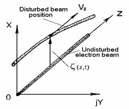
Fig. 4.1
Model of a filamentary electron beam
The solution will be sought in the form of the sum of two running waves with
right and left circular polarizations. Saving terminology (notations) of [21,22,2,6] we can write
where is
the electron propagation constant.
is
the electron propagation constant.
Here

Then


Let us represent the external transverse electrical field in the form of two
oscillations with right and left circular polarizations
Substituting (4.6)-(4.8) in the initial
equation (4.1)
gives

where  is
the cyclotron propagation constant.
is
the cyclotron propagation constant.
Note that:  since the functions
![]() depend
on the variable
depend
on the variable ![]() only.
only.
Therefore (4.9)
can be written as

In the undisturbed case ![]() the solution has the form
the solution has the form
Substituting this solution in (4.4) gives
Thus the motion of a
filamentary electron beam can be described by the sum of four circularly
polarized waves (transverse eigenmodes of the electron beam). Two waves with
the amplitudes ![]() are cyclotron waves, they have the opposite
polarizations and their phase velocities depend on the cyclotron frequency
are cyclotron waves, they have the opposite
polarizations and their phase velocities depend on the cyclotron frequency
 .
(4.13)
.
(4.13)
The other two waves with the
amplitudes ![]() are called synchronous waves, because their phase velocities
are equal (synchronous) to the electron beam velocity
are called synchronous waves, because their phase velocities
are equal (synchronous) to the electron beam velocity
The phase velocity of the wave with
the amplitude ![]() may be greater than the
longitudinal velocity of the electron beam and even become infinite in the case
of the cyclotron resonance (Fig. 4.2) Therefore
this wave was given the name fast
cyclotron wave of the electron beam. This wave can be either forward or
backward, depending on the phase velocity direction.
may be greater than the
longitudinal velocity of the electron beam and even become infinite in the case
of the cyclotron resonance (Fig. 4.2) Therefore
this wave was given the name fast
cyclotron wave of the electron beam. This wave can be either forward or
backward, depending on the phase velocity direction.
The phase velocity of the wave with the amplitude ![]() is
always smaller than the longitudinal velocity of the electron beam. Therefore
this wave is called a slow cyclotron wave of the electron beam. The phase velocity direction of
this wave is always positive, i.e. the wave is forward.
is
always smaller than the longitudinal velocity of the electron beam. Therefore
this wave is called a slow cyclotron wave of the electron beam. The phase velocity direction of
this wave is always positive, i.e. the wave is forward.
The synchronous waves ![]() differ by the directions
of their circular polarizations only, however, by analogy with cyclotron waves
they are often referred to as fast (
differ by the directions
of their circular polarizations only, however, by analogy with cyclotron waves
they are often referred to as fast (![]() ) and
slow (
) and
slow (![]() ) synchronous waves of the electron beam.
) synchronous waves of the electron beam.
Fig. 4.2
Dispersion characteristics of transverse waves.
FCW – Fast Cyclotron Wave, SCW- Slow Cyclotron
Wave,
SW – Fast and Slow Synchronous
Waves.
To clarify the structure of transverse waves it is convenient to use the system
of coordinates moving at the velocity ![]() (i.e.
the electron motion velocity) along the
(i.e.
the electron motion velocity) along the ![]() -axis. To do
so, it is sufficient to assume in (4.12) that
-axis. To do
so, it is sufficient to assume in (4.12) that ![]() .
.
Then
Thus, the amplitudes of the
synchronous waves (synchronous radius) describe the shift of the electron orbit
centers from the ![]() -axis. The amplitudes of the cyclotron waves determine the radius of the electron
rotations with the cyclotron frequency.
-axis. The amplitudes of the cyclotron waves determine the radius of the electron
rotations with the cyclotron frequency.
If
we imagine the situations when in the electron beam only one kind of waves is
excited consecutively, the beam configurations in all such cases will be
represented by spirals twisted spatially around the ![]() -
axis (Fig. 4.3).
Besides, for cyclotron waves each point (an electron) of such a spiral takes
part simultaneously in two motions, namely the rotation around the z-axis at
the angular frequency
-
axis (Fig. 4.3).
Besides, for cyclotron waves each point (an electron) of such a spiral takes
part simultaneously in two motions, namely the rotation around the z-axis at
the angular frequency ![]() and the movement along
the
and the movement along
the ![]() - axis at the velocity
- axis at the velocity ![]() . For synchronous waves there is no rotational motion, the electrons
are spatially shifted with respect to each other, thereby forming a spiral and
moving along the
. For synchronous waves there is no rotational motion, the electrons
are spatially shifted with respect to each other, thereby forming a spiral and
moving along the ![]() - axis only. In all cases the
beam trace (the intersection point of the beam at the plane
- axis only. In all cases the
beam trace (the intersection point of the beam at the plane ![]() =const) travels around a circle at the angular frequency
=const) travels around a circle at the angular frequency
![]() , with the rotation direction
being determined by the type of polarization.
, with the rotation direction
being determined by the type of polarization.
Thus, unlike waves of the space charge [1,23], in this case the grouping process is
connected only with a spatial curving of the electron beam without forming
bunches of the space charge.
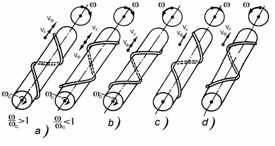
Fig. 4.3
a) - Fast forward and backward
Cyclotron
Waves,
b)
- Slow Cyclotron
Wave,
c) -
Synchronous Waves with right and left
polarizations.
(In all
cases the internal cylinder on which the electron beam
is
wound serves for the illustrative purpose only).
In the presence of an external electric field ![]() , the solution
of the initial system of equations (4.1),(4.2) may also be
sought in the form of the sum of four transverse waves having alternating
amplitudes
, the solution
of the initial system of equations (4.1),(4.2) may also be
sought in the form of the sum of four transverse waves having alternating
amplitudes

i.e.
![]() .
(4.17)
.
(4.17)
Here
 .
(4.18)
.
(4.18)
Since instead of one pair of
variables ![]() , two pairs of new
variables
, two pairs of new
variables ![]() are introduced, it
is necessary to impose some additional conditions to connect the members of
this new pair of variables. It is convenient to use the following
are introduced, it
is necessary to impose some additional conditions to connect the members of
this new pair of variables. It is convenient to use the following
 .
(4.19)
.
(4.19)
Then


Substituting these
expressions in (4.18)
and using (4.19)
gives


In the two limiting cases that of a
small transit angle and that of adiabatic
action of
electric fields on the electron beam the solution of this system of equations
can be simplified significantly.
In the first case, in the right-hand parts of the system of equations one can assume that
In the latter case, one can average the right-hand part of equations by the
period of cyclotron oscillations
Besides, when averaging, the wave
amplitudes ![]() should be taken to
be constant.
should be taken to
be constant.
Numerical integration of the system of equations (4.22), (4.23) is usually
straightforward and can be made using a personal computer.
In a more general case, when
It is also possible to represent
the initial equation of motion in the form

where
is the angular cyclotron frequency
and the longitudinal component of the magnetic flux density at the system axis,
respectively.
The solution can be readily found
for the cases when the longitudinal velocity of the electron beam does not
acquire modulation in time and dependents on the ![]() -coordinate
only, i.e.
-coordinate
only, i.e. ![]() .
.
Let us introduce  - the electron and cyclotron propagation constants,
respectively.
- the electron and cyclotron propagation constants,
respectively.
The solution is sought in the form of the sum of two waves with right and left
circular polarizations
 .
(4.30)
.
(4.30)
As before, the right-hand part of
equation (4.28)
is represented as
Using a procedure similar to that
employed above, we get
 .
(4.33)
.
(4.33)
In the presence of the external fields ![]() therefore
the solution will be sought in the form
therefore
the solution will be sought in the form
 .
(4.34)
.
(4.34)
Under the additional conditions
we obtain the system of
differential equations describing the behavior of transverse wave amplitudes
 .
(4.36)
.
(4.36)
In this case
Notes:
Applicability of the filamentary electron beam model.
The equations obtained are quite well applied for the electron beam of a
finite cross-section, if the external field phase changes negligibly across the
beam section
![]() ,
(4.39)
,
(4.39)
where ![]() is the electron beam radius,
is the electron beam radius, ![]() is the propagation constant of the wave of the
electrodynamics system.
is the propagation constant of the wave of the
electrodynamics system.
In practice, however, the
requirement ![]() is quite sufficient for
most issues.
is quite sufficient for
most issues.
V. Kinetic Powers of Transverse Waves
If a filamentary electron beam with the linear charge density ![]() is placed in the transverse electric field
is placed in the transverse electric field ![]() , the power of energy exchange between the electric field and
the electron beam element of the length dz is equal to
, the power of energy exchange between the electric field and
the electron beam element of the length dz is equal to
![]() ,
(5.1)
,
(5.1)
where ![]() ,
the sign * denotes the complex-conjugate value.
,
the sign * denotes the complex-conjugate value.
Besides
interaction with the transverse electric field, it is necessary to take into
account the interaction of the electron beam with a longitudinal electric field
![]() . To determine the value of
. To determine the value of ![]() , we use the quasi-stationary approximation [22]
, we use the quasi-stationary approximation [22]  , for which near the
 ![]() -axis
-axis
 ,
or
(5.2)
,
or
(5.2)
 , where
 ![]() .
(5.3)
.
(5.3)
Accordingly, the power of energy
exchange with the longitudinal field ![]() has
the form
has
the form
 .
(5.4)
.
(5.4)
The expression for the transverse
velocity can be given in the form
 ,
(5.5)
,
(5.5)
where ![]() means
the transverse velocity of the
electron beam trace in the plane
means
the transverse velocity of the
electron beam trace in the plane ![]()
Summing up the powers of the longitudinal
and transverse energy exchanges, we can write
 .
(5.6)
.
(5.6)
Now, we can use the representations
![]() ,
(5.7)
,
(5.7)
![]() ,
(5.8)
,
(5.8)
 ,
(5.9)
,
(5.9)
and, accordingly
![]() ,
, ![]() .
(5.10)
.
(5.10)
Substituting (5.7)-(5.10) into (5.6) and averaging
the power over the period ![]() , we get
, we get
Integrating (5.11)
over ![]() from 0 to
from 0 to ![]() , and taking into account that
, and taking into account that ![]() ,
we find
,
we find

The
expression between the braces under sing of integral depends only on the
coordinate ![]() , therefore the following
substitution was used
, therefore the following
substitution was used 
Now, choosing the integration
limits outside (before and after) the interaction
region, i.e. where the transverse electric field is equal to zero ![]() , we have
, we have

Let us first consider the simplest case
Then the equations for transverse wave
amplitudes have the form (4.36)-(4.38), i.e.,
Besides

We find ![]() from (5.17), (5.18), substitute
them into the expression for energy exchange power (5.13) and take
into account that
from (5.17), (5.18), substitute
them into the expression for energy exchange power (5.13) and take
into account that
![]() ,
(5.20)
,
(5.20)
![]() .
(5.21)
.
(5.21)
Then assuming that the electron
beam has no modulation at the input into the interaction region (i.e. ![]() ) we finally get
) we finally get
Thus, the period-averaged power of
energy exchange between the electron beam transverse waves and the external
electric fields is found equal to
where ![]() are
the current and the potential of the electron beam, respectively.
are
the current and the potential of the electron beam, respectively.
The positive sign of the kinetic power means that the power is added into the
electron beam at the excitation of a corresponding wave, and vice versa: the
negative sign implies that when a wave is excited the power is extracted from
the electron beam.
It is also possible to separate the transverse and longitudinal components of
the kinetic power, which are due to interactions with transverse and
longitudinal electric fields, respectively. For cyclotron waves the transverse
power is associated with rotation of electrons and, hence
 ,
(5.24)
,
(5.24)
then
 .
(5.25)
.
(5.25)
For synchronous waves the electron
beam has no transverse velocity, and hence
 .
(5.26)
.
(5.26)
Let us consider now a more general case when the static magnetic field varies along the ![]() - axis. In the paraxial approximation we can write
- axis. In the paraxial approximation we can write
where ![]() is the longitudinal component of the magnetic flux
density at the
is the longitudinal component of the magnetic flux
density at the ![]() -axis.
-axis.
In this case the equations of motion of an electron have the form
 ,
(5.28)
,
(5.28)
where  .
.
Accordingly, the equations
for transverse wave amplitudes are written as

Using a similar procedure and
substituting ![]() from (5.30), (5.31) into (5.13) and then
using (5.20), (5.21), we obtain the same result
from (5.30), (5.31) into (5.13) and then
using (5.20), (5.21), we obtain the same result
VI. Numerical Simulation and Helix-Type
Discretization
of the Injecting Electron Beam
To simplify the procedure of simulation, various configurations of ‘big charged
particles’ are usually used to analyze and to solve different issues of vacuum
microwave electronics since the middle of 60’s.
Transverse
interaction we are discussing is a 3D interaction because of the physical
principles of this one and the procedure of computer simulation must be also in
a 3D form. Nevertheless, in some
cases an essential simplification is
possible.
Let us start from the equation of
motion of a single electron having number “i”
 ,
(6.1)
,
(6.1)
or
![]() ,
(6.2)
,
(6.2)
Fields are calculated separately
![]() ,
(6.3)
,
(6.3)
where ![]() and
and
![]() are the electromagnetic
fields induced by electron beam,
are the electromagnetic
fields induced by electron beam, ![]() and
and ![]() are the microwave fields and
are the microwave fields and ![]() is
the external focusing magnetostatic field, respectively.
is
the external focusing magnetostatic field, respectively.
Let us assume ![]() and
and ![]() to be independent
variables, thereby making a transition from the description of the motion of
one electron to the description of the motion of a filamentary electron beam.
Then
to be independent
variables, thereby making a transition from the description of the motion of
one electron to the description of the motion of a filamentary electron beam.
Then
![]() ,
(6.4)
,
(6.4)
Such filamentary beams can be used
to describe the motion of a real beam of a finite cross-section.
** As an example, let us consider the case of the interaction
of circularly polarized slow-wave having
 .
(6.6)
.
(6.6)
and an electron beam of a finite
and round cross-section injecting along and coaxially the axis of this wave (
i.e., the ![]() - axes, see Fig. 6.1).
- axes, see Fig. 6.1).
We can choose the form of each
elementary (filamentary) beam as a helix inside the injecting electron beam (Fig. 6.1). Let us
choose the step of this helix as
 ,
(6.7)
,
(6.7)
where ![]() is
the longitudinal velocity of the injecting electron beam,
is
the longitudinal velocity of the injecting electron beam, ![]() is the angular frequency of the beam rotation under the
inner (radial) Coulomb forces.
is the angular frequency of the beam rotation under the
inner (radial) Coulomb forces.
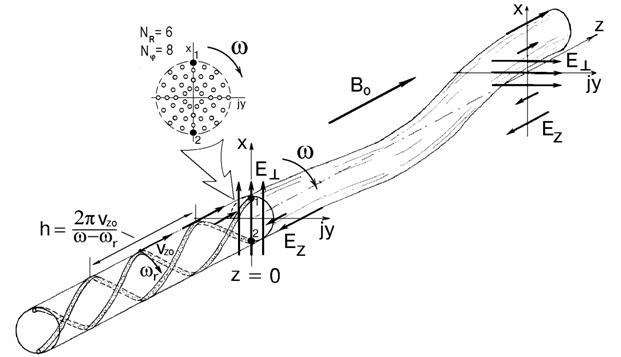
Fig. 6.1
Helix-type discretization of the injecting
electron beam
For the uniformly charged electron beam
 ,
,
 ,
(6.8)
,
(6.8)
where ![]() is the space charge density of the injecting electron
beam.
is the space charge density of the injecting electron
beam.
In the case we are discussing, the
cross-point of each elementary (filamentary) beam at the plane ![]() is rotating at the angular frequency
is rotating at the angular frequency ![]() and each such beam has stationary (concerning the fields of this
circularly polarized wave) boundary (at
and each such beam has stationary (concerning the fields of this
circularly polarized wave) boundary (at ![]() ) conditions
and as a result of it
) conditions
and as a result of it
for any beam and everywhere inside
the interaction region (![]() is the linear charge
density of this filamentary beam).
is the linear charge
density of this filamentary beam).
The
boundary condition of the uniform charged electron beam are given by
where
![]() ,
,
![]()
![]() .
.
![]() - radius of the injecting electron beam,
- radius of the injecting electron beam,
![]() - number of elementary beams
on each ring,
- number of elementary beams
on each ring,
![]() - number of rings,
- number of rings,
![]() - total number of elementary beams ( 50-150 usually ),
- total number of elementary beams ( 50-150 usually ),
 ,
, 
Using
continuity
equation
 ,
(6.12)
,
(6.12)
one can
write for each elementary beam
Thus,
firstly:
![]() ,
(6.14)
,
(6.14)
where ![]() ,
, ![]() are the space charge linear along z-axes density
and the longitudinal velocity of the elementary beam, respectively.
are the space charge linear along z-axes density
and the longitudinal velocity of the elementary beam, respectively.
And secondly: the simulation may be
fulfilled at any fixed moment of time. Any changing in time is
completely equal to the rotation of the system around z-axis (see Fig. 6.1). In
all equations

for
transverse coordinates and transverse velocities of any elementary beam.
It is important to emphasize that all restrictions on
helix-form of each elementary beam are essential only for the injecting beam (![]() ). Inside
the interaction region (z>0) the motion of each elementary beam can be
absolutely arbitrary and the electron beam interaction includes both the transverse
grouping and the longitudinal one.
). Inside
the interaction region (z>0) the motion of each elementary beam can be
absolutely arbitrary and the electron beam interaction includes both the transverse
grouping and the longitudinal one.
** It is also important to emphasize that instead of (6.6), any type of
electromagnetic fields rotating around ![]() -axes at the
angular frequency
-axes at the
angular frequency ![]() can be also used here.
can be also used here.
Coulomb
fields of the electron beam can be found using approximate formulas (see
Appendix)

where:
![]() is equal to 1/2 of the min distance between partial beams
at
is equal to 1/2 of the min distance between partial beams
at ![]() .
.
** As an another example, let us consider the case when the
electron beam having some initial rotation around ![]() -axes
is injected to the region with axially-symmetric and space-variable magnetic
(or electric) static field
-axes
is injected to the region with axially-symmetric and space-variable magnetic
(or electric) static field
where![]() is
the longitudinal component of the magnetic flux density at the
is
the longitudinal component of the magnetic flux density at the ![]() -axis.
-axis.
Boundary
conditions in such case
or

![]() ;
;
![]()
Where![]() are
the radius and the phase of the initial rotation of the electron beam, i.e. of
each electron of the beam ( at z = 0 and t =
0 ).
are
the radius and the phase of the initial rotation of the electron beam, i.e. of
each electron of the beam ( at z = 0 and t =
0 ).
Therefore, all main consequences of helix-type discretization (6.11), (6.14) and (6.15) exist in
this case also.
** We could also consider the case when the electron beam
having some initial rotation around ![]() -axes is
injected into the region with electromagnetic fields rotating around
-axes is
injected into the region with electromagnetic fields rotating around ![]() -axes at the angular frequency
-axes at the angular frequency![]() and so
on.
and so
on.
Helix-type discretization of the injecting electron beam has been carefully
tested and successfully used by different authors [4-8, 25, etc.].
VII. Discussion
In the simplest case transverse waves of the electron beam can be analyzed by
comparing them with the space charge waves in order to reveal the potential
advantages that could be realized when using transverse grouping in electron
beams.
Let us outline some of them briefly:
·
In
contrast to
space charge waves*, phase velocities of transverse waves are independent of
the reduced value of the plasma frequency (which is not constant
along and across the electron beam and is also dependent nonlinearly on the
signal amplitude) and, consequently, it is now possible to make the synchronism
of the transverse wave interaction with external fields incomparably more
stable. For the same reason, devices based on interaction with transverse waves
must have phase-frequency characteristics with a considerably improved
linearity.
·
No
restrictions were
imposed on the signal amplitude value when the equations for transverse waves
were derived. On the other hand, for the space charge waves the restrictions of
the modulation depth are essential. Hence, one can also expect a higher
linearity of the amplitude characteristics in energy exchange with transverse
waves of the electron beam.
·
Transverse
waves of the
electron beam are circularly polarized, that provides an additional possibility
to select waves taking part in energy exchange, thereby making it possible to
improve the quality of interaction.
·
At
the point of
cyclotron resonance (![]() ) the phase velocity of the
fast cyclotron wave becomes infinite in contrast to phase velocities of other
waves. Therefore just with this wave in a plane transverse and uniform
electrical field of the resonator it is possible to carry out an efficient
prolonged (
) the phase velocity of the
fast cyclotron wave becomes infinite in contrast to phase velocities of other
waves. Therefore just with this wave in a plane transverse and uniform
electrical field of the resonator it is possible to carry out an efficient
prolonged (![]() >>1) interaction to ensure
a high efficiency of signal power transmission from the resonator to the wave
and vice versa.
>>1) interaction to ensure
a high efficiency of signal power transmission from the resonator to the wave
and vice versa.
·
A
slow synchronous
wave has a negative kinetic power, a phase velocity equal to the electron beam
velocity and is not connected with excitation of transverse velocities of the
beam electrons. The interaction with this wave must be more efficient than with
the space charge slow wave and provide a single velocity character of the spent
electron beam, i.e. it allows an extensive recovery of the spent beam energy.
In such energy exchange of the running circularly polarized wave with the field
the phase-frequency characteristics must have a higher linearity.
·
Some
additional
information [12-14]
is available via Internet :
http://jre.cplire.ru/jre/aug99/1/text.html,
http://jre.cplire.ru/jre/sep99/1/text.html,
http://jre.cplire.ru/jre/oct99/1/text.html .
*) The phase velocities of the fast
(+) and slow (-) waves of the space charge are known [1,23] to be equal to: ![]() , respectively, where
, respectively, where ![]() - is
the reduced value of the plasma frequency in the electron beam.
- is
the reduced value of the plasma frequency in the electron beam.
VIII. Selected Bibliography
[1] V.M.Lopukhin et al,
“Noises and Parametric Phenomena in Electron Beams”, Nauka, Moscow,
1966. (In Russian).
[2] V.A.Vanke et al,
“Super Noiseless Cyclotron-Wave Amplifiers”, Soviet Physics Uspekhi,
May-June 1970, vol. 12, No. 6, p. 743.
[3] V.I.Yuriev et al,
“Experimental Study of the Interaction of Synchronous Waves of the Electron
Beam and Travelling Wave of the Electrodynamics System”, Radiotechnique
& Electronics, 1972, vol. 17, No. 4, p. 830. (In Russian).
[4] A.A.Zaitzev, “On the
Efficiency of the Interaction of Transverse Waves of the Electron Beam and
Electromagnetic Fields”, Ph.D. thesis, Faculty of Physics, Moscow State
University, 1979. (in Russian).
[5] V.A.Vanke et al,
“The Results of the Investigations of the Circularly Polarized TWT and their
Analysis”, Radiotechnique & Electronics, 1981, vol. 26, No. 11, p.
2365. (In Russian).
[6] V.A.Vanke, “The
Interaction of the Oscillations and Waves of the Electron Beam and
Electromagnetic Fields”, D.Sc. thesis, Faculty of Physics, Moscow State University, 1981. (in Russian).
[7] V.I.Gorelikov, “The
Efficiency of the Excitation and Conversion of Fast Cyclotron Waves in High
Power Electron Beams”, Ph.D. thesis, Faculty of Physics, Moscow State
University, 1984. (in Russian).
[8] A.V.Konnov, “The
Interaction of Circularly Polarized Electromagnetic Slow Waves and Transverse
Synchronous Wave of the Electron Beam”, Ph.D. thesis, Faculty of
Physics, Moscow State University, 1988. (in Russian).
[9] Yu.A.Budzinsky,
S.P.Kantyuk, “A New Class of Self-Protecting Low-Noise Microwave Amplifiers”,
Proc. IEEE MTT-S Microwave Symposium, Atlanta, USA, June 1993,
Digest, vol. 2, p. 1123.
[10] S.V.Bykovsky, “Theory of
the Energy Exchange Processes of Transverse Waves of the Electron Beam and the
Development Basing on this Theory of Cyclotron Wave Protectors with Brief
Recovery Time of Around 10 ns”, Ph.D. thesis, The Istok Corporation,
Fryazino, Moscow region, 1996.
[11] I.A.Boudzinski et al, “Microwave Devices Using Fast Cyclotron
Wave”, Radiotechnique, 1999, No. 4, p. 32. (In
Russian).
[12] Vanke V.A., “Microwave
Electronics Based on Electron Beam Transverse Waves Using
(State-of-the-Art and Perspectives. Russian Experience)”, Journal of
Radioelectronics, 1999, No. 8: http://jre.cplire.ru/jre/aug99/1/text.html.
[13] Vanke V.A. et al, “High Power Converter of Microwaves
into DC”, Journal
of Radioelectronics, 1999, No. 9: http://jre.cplire.ru/jre/sep99/1/text.html.
[14] Vanke V.A. et al, “Cyclotron Wave Electrostatic
Amplifier”, Journal
of Radioelectronics, 1999, No. 10: http://jre.cplire.ru/jre/oct99/1/text.html.
[15] V.A.Vanke, “Microwave
Electronics Based on Electron Beam Transverse Waves Using” (Invited), Technical
Report of the Institute of Electronics, Information and Communication Engineers
(Japan), ED99-247, 1999, p. 1.
[16] I.A.Boudzinski,
S.V.Bykovski, “Amplifying and Protective Devices Based on Electron Beam Fast
Cyclotron Wave”, Proc of the 2nd International
Vacuum Electronics Conference,
April 2-4, 2001, Noordwijk, The Netherlands, p. 153.
[17] R.Adler et al, “Excitation and Amplification of Cyclotron
Waves and Thermal Orbits in the Presence of Space Charge “, J.
Appl. Phys., 1961, vol. 32, No. 4, p. 672.
[18] V.A.Vanke,
V.B.Magalinsky, “On the Role of Space Charge at the Amplification of Intrinsic
Noise Orbits in High-Frequency Quadrupole Field”, Higher School Reports,
ser. Radiophysics, 1966, vol. 9, No. 5, p. 831. (in Russian).
[19] P.L.Kapitza, “High-Power
Electronics”, Edition of the USSR Academy of Sciences, 1962, vol. 1, ch.
1. (in Russian).
[20] N.N.Bogolyubov,
Yu.A.Mitropol’skii, Asymptotic Methods in the Theory of Nonlinear Oscillations,
Fizmatgiz, 1963. (in Russian).
[21] V.Dubravec, “Wave Theory
of Cuccia Couplers”, Arch. Elektr. Ubertrag., 1964, vol. 18, No.
10, p. 585, (in German).
[22] V.Dubravec, “General
Power Relations of Cyclotron Waves”, Electron. Commun., 1964, vol. 39,
No. 4, p. 558.
[23] W.H. Louisell, "Coupled
Mode and Parametric Electronics," John Wiley & Sons, Inc., New
York, London, 1960.
[24] G.A.Sukach, “On the
Calculation of the Space Charge Field”, Vestnik KPI, ser.
Radiotechnique & Electronics, 1970, No.7, p. 59. (in Russian).
[25] A.Kita, “Study of the
Conversion Region in CWC via Computer Experiment”, MS thesis, The
Graduate School of Engineering, Kyoto University, 1998. (in Japanese)
IX. Appendix
(Coulomb Fields)
In many cases
![]()
![]() ,
(9.1)
,
(9.1)
where: ![]() ,
, ![]() are the radius of the
electron beam and the radiuses of curvature of the elementary (filamentary)
beams, respectively.
are the radius of the
electron beam and the radiuses of curvature of the elementary (filamentary)
beams, respectively.
In such cases we can simplify the task and calculate the electric field of a
charged rod placing it along the tangent of the elementary beam.
Let us
consider three coordinate systems (Fig. 9.1)
![]()
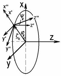
Fig. 9.1
The ![]() -
axes is the tangent (charged rod) of the elementary beam having the cross-point
coordinate
-
axes is the tangent (charged rod) of the elementary beam having the cross-point
coordinate ![]() at the plane
at the plane ![]() .
.
We can write for the electric field of such charged rod at the point ![]()

Where ![]() are the linear charge density of the rod and the
dielectric constant, respectively.
are the linear charge density of the rod and the
dielectric constant, respectively.
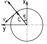
Fig. 9.2
In compliance with Fig. 9.1 and Fig. 9.2 one can
write the coordinate transformation formulas

and

Using (9.2)-(9.5) one can obtain
(6.16).
A small add ![]() in
(6.16) is a
rational way to avoid mathematical singularities
in
(6.16) is a
rational way to avoid mathematical singularities
when ![]() [24].
[24].
**************************
|
|
|